Download
1 / 20
220 likes | 478 Vues
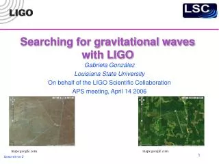
Search for Stochastic Gravitational Waves with LIGO. XLII nd Rencontres de Moriond Albert Lazzarini (on behalf of the LIGO Scientific Collaboration) La Thuile, Val d'Aosta, Italy March 11-18, 2007. NASA/WMAP Science Team. Outline. Stochastic gravitational waves Sources

E N D
Search for Stochastic Gravitational Waves with LIGO XLIInd Rencontres de Moriond Albert Lazzarini (on behalf of the LIGO Scientific Collaboration) La Thuile, Val d'Aosta, Italy March 11-18, 2007 NASA/WMAP Science Team
Outline • Stochastic gravitational waves • Sources • Characterization of strain • Search techniques • All-sky averaged search • Spatially resolved map • Recent observational results • Prospects LIGO Laboratory at Caltech
Stochastic gravitational wave background Analog from cosmic microwave background -- WMAP 2003 • GWs are the able to probe the very early universe g • Search for a GW background by cross-correlating interferometer outputs in pairs • US-LIGO : Hanford, Livingston • Europe: GEO600, Virgo • Japan: TAMA • Good sensitivity requires: • GW > 2D (detector baseline) • f < 40 Hz for LIGO pair over 3000 km baseline • Good low-f sensitivity and short baselines LIGO Laboratory at Caltech
Stochastic signals Cosmological processes • Inflation -- flat spectrum (Turner) • Phase transitions -- peaked at phase transition energy scale (Kamionkowski) • Cosmic strings -- gradually decreasing spectrum (Damour & Vilenkin) • Pre big-bang cosmology -- rising strength with f (Buonanno et al.) Astrophysical Foregrounds • Incoherent superposition of many signals from various signal classes (Ferrari, Regimbau) • Coalescing binaries • Supernovae • Pulsars • Low Mass X-Ray Binaries (LMXBs) • Newly born neutrons stars • Normal modes - R modes • Binary black holes • Black hole ringdowns • Gaussian -> non-Gaussian (“popcorn” noise) depending on rates Drasco & Flannigan, Phys.Rev. D67 (2003) • Spectra follow from characteristics of individual sources -- e.g., spatial anisotropy for nearby (foreground) contributors LIGO Laboratory at Caltech
Characterization of a Stochastic Gravitational Wave Background • GW energy density given by time derivative of strain • Assuming SGWB is isotropic, stationary and Gaussian, the strength is fully specified by the energy density in GWs • f) in terms of a measurable strain power spectrum, Sgw(f): • Strain amplitude scale: Allen & Romano, Phys.Rev. D59 (1999) LIGO Laboratory at Caltech
Technique -- Sky-averaged searchTime-independent Detection Strategy • Cross-correlation statistic: • Optimal filter: • Make many (N~ 104) repeated short (T = 60s) measurements to track instrumental variations: 4all-sky averaged result penalizes high frequencies for non-colocated detectors (f) LIGO Laboratory at Caltech
Sensitivities of LIGO interferometers during S422 February - 23 March 2005 improves sensitivity reach over individual noise floors. H1 - L1: 353.9 hr H2 - L1: 332.7 hr. Scheduled for publication March 2007 : ApJ 658 (2007) LIGO Laboratory at Caltech
Run Averaged Coherences: A measure of intrinsic sensitivity H1 - L1 Distribution of coherence follows expected exponential PDF 1 Hz comb due to GPS timing pulse 1/N noise floor H2 - L1 16 Hz Data Acq. + injected lines LIGO Laboratory at Caltech
Histogram of normalized measurement residuals Tobs = 353.9 hr Nseg = 12637(after cuts) • Make a measurement every 192s • Look at statistics of measurements to determine whether they are Gaussian LIGO Laboratory at Caltech
90% Bayesian upper limit vs. spectral index, All-sky averaged results for S4 S4 result: 0 < 6.5 x 10⁻⁵ (90% U.L.) Optimally combined spectrum: H1 - L1 & H2 - L1 H1 - L1: 353.9 hr; Nseg = 12,637 H2 - L1: 332.7 hr; Nseg = 11,849 Standard deviation of measurement Modulation of envelope due to (f) • Scheduled for publication in ApJ 658 (March 2007) H1 - L1 Evolution of measurement over time LIGO Laboratory at Caltech
Tests with signal injectionsHardware & Software injected = 1.1 x 10⁻² • HW: Introduce coherent excitation of test masses (WA - LA) with a spectrum simulation a constant GW(f) background with different strengths • SW: Simulated signal added to strain signal Time-lag shifts of injected signal LIGO Laboratory at Caltech
The Stochastic GW Landscape ApJ 658 (2007) PRD 69 (2004) 122004 H0 = 72 km/s/Mpc Armstrong, ApJ 599 (2003) 806 PRL 95 (2005) 221101 Smith et al., PRL 97 (2006) 021301 Kolb & Turner, The Early Universe (1990) Jenet et al., ApJ 653 (2006) 1571 (Tobs = 1 yr) (Tobs = 1 yr) Allen&Koranda, PRD 50 (1994) 3713 Damour & VilenkinPRD 71 (2005) 063510 Buonanno et al.,PRD 55 (1997) 3330 Gasperini & Veneziano, Phys. Rep. 373 (2003) 1 Turner,PRD 55 (1997) 435 LIGO Laboratory at Caltech
Model of Damour & Vilenkin p: probability for reconnection G: string tension - regime accessible by LIGO : loop size - regime accessible by LIGO S4 all-sky observationsImplications for Cosmic strings BBN Pulsar timing Tobs = 1 yr DesignTobs = 1 yr DesignTobs = 1 yr LIGO Laboratory at Caltech
Spatially-resolved searchTime-dependent Detection Strategy • Time-dependent overlap reduction function tracks a point in the sky over the sidereal day: • Time dependent optimal filter enables spatially resolved measurement: Point spread function of antenna • Characteristic size of point spread function: • /D • ~ 11o @ 500 Hz for D = 3000 km • Diffraction-limited GW astronomy LIGO Laboratory at Caltech
Spatially resolved search with S4Simulations & Validation Detection of an injected hardware pulsar simulation LIGO Laboratory at Caltech
Upper limit sky mapsNo detection of signal at S4 sensitivity Submitted to PRD; arXiv:astro-ph/0701877v1 • GW(f) ~ const Results • Integration over sky yields sky-averaged result that is consistent with the all-sky technique within measurement errors • Distribution of signal consistent with Gaussian PDF with 100 DOFs (# of independent sky patches) • 90% Bayesian UL:GW < 1.02 x 10⁻⁴ • GW(f) ~ f3 Results • Distribution of signal consistent with Gaussian PDF with 400 DOFs (# of indpendent sky patches) • 90% Bayesian UL:GW (f) < 5.1 x 10⁻⁵ (f/100Hz)3 LIGO Laboratory at Caltech
Use spatially resolved stochastic search technique to look for periodic emissions of unknown f:Sco-X1 Template-less search: use signal in one detector as the “template” LIGO Laboratory at Caltech
Summary - S4 results • All-sky measurement: h722 < 6.5 x 10⁻⁵ • 13X improvement over previous (S3) result • Still weaker than existing BBN limit • S4 (and previous S3) are starting to explore, restrict parameter space of some stochastic models, such as cosmic strings and pre-big bang • The S5 data analysis is in progress -- should beat the BBN limits for models in which signal is concentrated in the LIGO band • Spatially resolved measurements: • New technique that exploits phased-array nature of the LIGO site pairs to steer beam and to track sky positions • All-sky result follows as a subset of the measurements • Approach can be used look for a number of astrophysical foregrounds, by changing the optimal filter to match the source properties • Work ongoing to (i) implement deconvolution of antenna point spread function from raw maps; (ii) decompose map into spherical harmonics basis functions, analogous to CMB maps. • Expected sensitivities with one year of data from LLO-LHO: • Initial LIGO h2 < 2x10⁻⁶ • Advanced LIGO h2 < 7x10⁻¹⁰ LIGO Laboratory at Caltech
FINIS LIGO Laboratory at Caltech
Irinsic Sensitivity:Y Trend for Entire Run Tobs = 353.9 hr Nseg = 12,637(after cuts) LIGO Laboratory at Caltech