Download

1 / 26
280 likes | 441 Vues
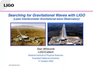
Direct Searches for Stochastic Gravitational Waves with LIGO: status and prospects. Albert Lazzarini California Institute of Technology On behalf of the LIGO Scientific Collaboration The 11 th International Symposium on Particles, Strings and Cosmology 30 May 2005 Gyeongju, Korea.

E N D
Direct Searches for Stochastic Gravitational Waves with LIGO: status and prospects Albert Lazzarini California Institute of Technology On behalf of the LIGO Scientific Collaboration The 11th International Symposium on Particles, Strings and Cosmology 30 May 2005 Gyeongju, Korea Black Holes courtesy of NCSA
Outline of Presentation • Stochastic gravitational waves • Characterization of strain • Sources • LIGO Concept • Principle of operation • Sites, facilities • Sensitivity • Recent observational results • Prospects LIGO Laboratory at Caltech
Stochastic gravitational wave background Analog from cosmic microwave background -- WMAP 2003 The integral of [1/f•GW(f)] over all frequencies corresponds to the fractional energy density in gravitational waves in the Universe • GWs are the able to probe the very early universe • Detect by cross-correlating interferometer outputs in pairs • US-LIGO : Hanford, Livingston • Europe: GEO600, Virgo • Japan: TAMA • Good sensitivity requires: • GW > 2D (detector baseline) • f < 40 Hz for LIGO pair over 3000 km baseline • Initial LIGO limiting sensitivity (1 year search): <10-6 LIGO Laboratory at Caltech
Cosmological Gravitational Waves • • Terrestrial LIGO Laboratory at Caltech
Characterization of a Stochastic Gravitational Wave Background • GW energy density given by time derivative of strain • Assuming SGWB is isotropic, stationary and Gaussian, the strength is fully specified by the energy density in GWs • f) in terms of a measurable strain power spectrum, Sgw(f): • Strain amplitude scale: Allen & Romano, Phys.Rev. D59 (1999) LIGO Laboratory at Caltech
Stochastic signals fromcosmological processes • Inflation -- flat spectrum • Kolb & Turner, The Early Universe • Phase transitions -- peaked at phase transition energy scale • Kamionkowski, Kosowski & Turner, Phys.Rev. D49 (1994) • Apreda et al., Nucl.Phys. B631 (2002) • Cosmic strings -- gradually decreasing spectrum • Damour & Vilenkin , Phys.Rev. D71 (2005) • Pre big-bang cosmology • Buonanno, Maggiore & Ungarellli , Phys.Rev. D55 (1997) LIGO Laboratory at Caltech
Stochastic signals fromastrophysical processes • Incoherent superposition of many signals from various signal classes • Coalescing binaries • Supernovae • Pulsars • Low Mass X-Ray Binaries (LMXBs) • Newly born neutrons stars • Normal modes - R modes • Binary black holes • Gaussian -> non-Gaussian (“popcorn” noise) depending on rates Drasco & Flannigan, Phys.Rev. D67 (2003), • Spectra follow from characteristics of individual sources Maggiore, Phys.Rept. 331 (2000) LIGO Laboratory at Caltech
The Cosmological Gravitational Wave “Landscape” Kolb & Turner, The Early Universe (1990) Range of Interferometers (Ground & Space-Based Lommen, astro-ph/0208572 n & Koranda, PRD 50 (1994) Armstrong et al., ApJ 599 (2003) LIGO Laboratory at Caltech
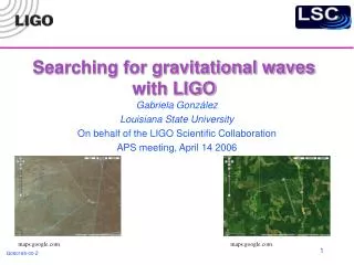
The LIGO Laboratory Sites Interferometers are aligned along the great circle connecting the sites Hanford, WA MIT 3002 km (L/c = 10 ms) Caltech Livingston, LA LIGO Laboratory at Caltech
The LIGO Observatories GEODETIC DATA (WGS84) h: -6.574 m X arm: S72.2836°W : N30°33’46.419531” Y arm: S17.7164°E : W90°46’27.265294” Livingston Observatory Louisiana One interferometer (4km) Hanford Observatory Washington Two interferometers(4 km and 2 km arms) GEODETIC DATA (WGS84) h: 142.555 m X arm: N35.9993°W : N46°27’18.527841” Y arm: S54.0007°W : W119°24’27.565681” <- Livingston, LA Hanford, WA -> LIGO Laboratory at Caltech
Detector concept Light makes Nb bounces h = L/L => / = 2 Nb hL/ • The concept is to compare the time it takes light to travel in two orthogonal directions transverse to the gravitational waves. • The gravitational wave causes the time difference to vary by stretching one arm and compressing the other. • The interference pattern is measured (or the fringe is split) to one part in 1010, in order to obtain the required sensitivity. LIGO Laboratory at Caltech
LIGO First Generation DetectorLimiting noise floor • Interferometer sensitivity is limited by three fundamental noise sources • seismic noise at the lowest frequencies • thermal noise (Brownian motion of mirror materials, suspensions) at intermediate frequencies • shot noise at high frequencies • Many other noise sources lie beneath and must be controlled as the instrument is improved LIGO Laboratory at Caltech
The LIGO is Approaching its Design Sensitivity factor 2X of design goal throughout LIGO band LIGO Laboratory at Caltech
Detection strategy • Spectrum: • Cross-correlation statistic: • Optimal filter (assume gw(f) = const): • Make many (N~ 104) repeated short (T = 60s) measurements to track instrumental variations: LIGO Laboratory at Caltech
(f) - Overlap reduction factor g(f) LIGO Laboratory at Caltech
S2 H1-L1 results using previously outlined method • Scatter plot of normalized residuals vs. • Distribution of over S2 run LIGO Laboratory at Caltech
S3 Expected Sensitivity: H1-L1 Estimated error of measurement (+3) plotted for the H1-L1 pair as a function of run time. Preliminary LIGO Laboratory at Caltech
Current and expected results on gw h1002 LIGO Laboratory at Caltech
The Cosmological Gravitational Wave “Landscape” LIGO Laboratory at Caltech
Frequency range for GW Astronomy Audio band Terrestrial Space Dynamic range of Gravitational Waves • Terrestrial and space detectors complementary probes • Provide ~8 orders of magnitude coverage LIGO Laboratory at Caltech
Initial and Advanced LIGO LIGO Laboratory at Caltech
The Cosmological Gravitational Wave “Landscape” LIGO Laboratory at Caltech
Growing International Network of GW Interferometers LISA GEO: 0.6km On-line VIRGO: 3km 2005 - 2006 LIGO-LHO: 2km, 4km On-line TAMA: 0.3km On-line LIGO-LLO: 4km On-line AIGO: (?)km Proposed • Operated as a phased array: • - Enhance detection confidence • - Localize sources • - Decompose the polarization of gravitational waves • - Precursor triggers from low frequency LIGO Laboratory at Caltech
Summary • The current best published IFO-IFO upper-limit is from S1:h2 < 23+/-4.6 • S2 result: 0.018 (+0.007- 0.003) PRELIMINARY • The S3 data analysis is in progress. Expect: < few x 10-4 • H1-H2 is the most sensitive pair, but it also suffers from cross-correlated instrumental noise. • Also working on: • Set limits for gw(f) ~ n(f/f0)n • Targeted searches (astrophysical foregrounds, spatially resolved map) • Expected sensitivities with one year of data from LLO-LHO: • Initial LIGO h2 < 2x10⁻⁶ • Advanced LIGO h2 < 7x10⁻¹⁰ LIGO Laboratory at Caltech
FINIS LIGO Laboratory at Caltech
What is known about the stochastic gravitational wave background? Allen & Koranda, PhysRevD Lommen, astro-ph/0208572 Kolb & Turner, TheEarlyUniverseAddisonWesley1990 2 LIGO Laboratory at Caltech