Download
1 / 10
100 likes | 245 Vues
Simulated real beam into simulated MICE. Mark Rayner CM26. Introduction. Various fancy reweighting schemes have been proposed But how would the raw beam fare in Stage 6? TOF0 measures p x and p y at TOF1 given quadrupole field maps

E N D
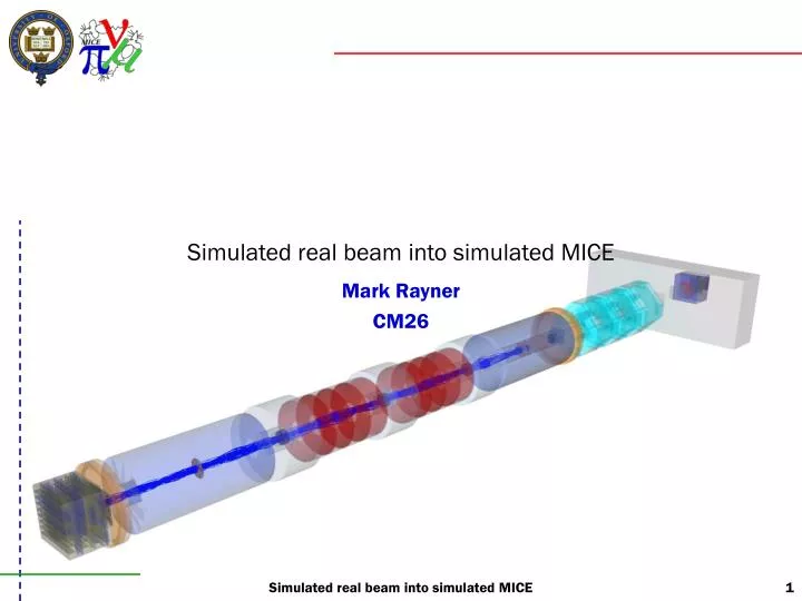
Simulated real beam into simulated MICE Mark Rayner CM26 Simulated real beam into simulated MICE
Introduction • Various fancy reweighting schemes have been proposed • But how would the raw beam fare in Stage 6? • TOF0 measures px and py at TOF1 given quadrupole field maps • On Wednesday I described the measurement of a 5D covariance matrix (x,px,y,py,pz) • In this talk, compare two monochromatic 6-200 beams in Stage 6 • A matched beam in the tracker • A measured beam at TOF1 • Measured (x, px) and (y, py) covariances • No dispersion Simulated real beam into simulated MICE
Time in MICE • RF frequency = 200 MHz, period = 5 ns • Neutrino factory beam • Time spread is approximately 500 ps • Want < 50 ps resolution in cavities • Possible methods for tracking time from TOF1 to the upstream tracker • Use of the adiabatic invariant pperp2/Bz0 • The flux enclosed by the orbit of a charged particle in an adiabatically changing magnetic field is constant • Use of the linear transfer matrix for solenoidal fields • Multiply matrices corresponding to slices with varying Bz0 and kappa • Tracking step-wise through a field map • Measured or calculated? • A Kalman filter • Implemented between the trackers • Static fields • None of these methods is particularly difficult • Nevertheless, there is merit in simplicity • This talk will investigate the first approach • Is pperp2/Bz0 really an adiabatic invariant in the MICE Stage 6 fields? Simulated real beam into simulated MICE
Reconstruction procedure Track through through each quad, and calculate s»leff + dF + dD zTOF1 – zTOF0 = 8 m Assume the path length S»zTOF1 – zTOF0 Q5 Q6 Q7 Q8 Q9 TOF0 TOF1 Estimate the momentum p/E = S/Dt Add up the total path S = s7 + s8 + s9 + drifts Calculate the transfer matrix Deduce (x’, y’) at TOF0 from (x, y) at TOF1 Deduce (x’, y’) at TOF1 from (x, y) at TOF0 Simulated real beam into simulated MICE
B field and beta lattice matched in tracker babs = 42cm Simulated real beam into simulated MICE
Matched beam Simulated real beam into simulated MICE
Beam 1 • Beam 1: Runs 1380 – 1393 • Kevin’s optics 6 mm – 200 MeV/c emittance-momentum matrix element • Analysis with TOF0 and TOF1 – the beam just before TOF1: • Covariances: • sigma(xpx) = –610 mm MeV • sigma(ypy) = +85 mm MeV • Longitudinal momentum • Min. ionising energy loss in TOF1 = 10.12 MeV • pz before 7.5 mm diffuser (6-200 matrix element) = 218 MeV [Marco] • RF cavities have gradient 9.1 MV/m and 90 degree phase for the reference muon • Start with pz = N(230, 0.1) MeV before TOF1, centred beam, transverse optics as above Simulated real beam into simulated MICE
Measured beam Simulated real beam into simulated MICE
Matching time in the first cavity • Sigma pz = 24.5 MeV • Beta = 0.857 to 0.904 (-1s to +1s) • Time over L = 17.2 ns to 16.3 ns • Difference = 0.89 ns • RF period = 5 ns • Transfer matrix: • Work the covariance matrix back from the 1st RF to before the TOF: • L/Eref = 4423 mm / (230 MeV * 300 mm/ns) = 0.064 ns/MeV • Sigma t RF = 500 ps • Sigma t = sqrt( (0.5 ns)**2 + (1.568 ns)**2 ) = 1.645 ns • Cov(t,pz) = –38.42 ns MeV Simulated real beam into simulated MICE
Conclusion Simulated real beam into simulated MICE