Simulated Annealing: Iterative Improvement for Combinatorial Optimization
170 likes | 226 Vues
Learn the principles and methods of Simulated Annealing to solve optimization problems efficiently, including Iterative Improvement and Markov Chains. Understand how to cope with disadvantages and enhance performance.

Simulated Annealing: Iterative Improvement for Combinatorial Optimization
E N D
Presentation Transcript
Simulated Annealing Van Laarhoven, AartsVersion 1, October 2000
Iterative Improvement 1 • General method to solve combinatorial optimization problems Principle: • Start with initial configuration • Repeatedly search neighborhood and select a neighbor as candidate • Evaluate some cost function (or fitness function) and accept candidate if "better"; if not, select another neighbor • Stop if quality is sufficiently high, if no improvement can be found or after some fixed time
Iterative Improvement 2 Needed are: • A method to generate initial configuration • A transition or generation function to find a neighbor as next candidate • A cost function • An Evaluation Criterion • A Stop Criterion
Iterative Improvement 3 Simple Iterative Improvement or Hill Climbing: • Candidate is always and only accepted if cost is lower (or fitness is higher) than current configuration • Stop when no neighbor with lower cost (higher fitness) can be found Disadvantages: • Local optimum as best result • Local optimum depends on initial configuration • Generally no upper bound on iteration length
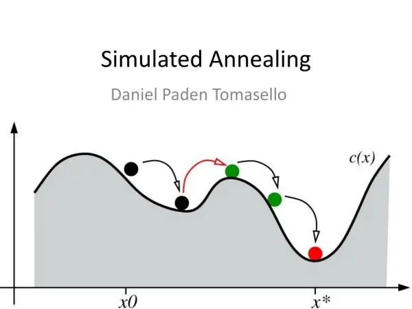
How to cope with disadvantages • Repeat algorithm many times with different initial configurations • Use information gathered in previous runs • Use a more complex Generation Function to jump out of local optimum • Use a more complex Evaluation Criterion that accepts sometimes (randomly) also solutions away from the (local) optimum
Simulated Annealing Use a more complex Evaluation Function: • Do sometimes accept candidates with higher cost to escape from local optimum • Adapt the parameters of this Evaluation Function during execution • Based upon the analogy with the simulation of the annealing of solids
Other Names • Monte Carlo Annealing • Statistical Cooling • Probabilistic Hill Climbing • Stochastic Relaxation • Probabilistic Exchange Algorithm
Analogy • Slowly cool down a heated solid, so that all particles arrange in the ground energy state • At each temperature wait until the solid reaches its thermal equilibrium • Probability of being in a state with energy E : Pr { E = E } = 1/Z(T) . exp (-E / kB.T) E Energy T Temperature kB Boltzmann constant Z(T) Normalization factor (temperature dependant)
Simulation of cooling (Metropolis 1953) • At a fixed temperature T : • Perturb (randomly) the current state to a new state • E is the difference in energy between current and new state • If E < 0(new state is lower), accept new state as current state • If E 0, accept new state with probability Pr (accepted) = exp (- E / kB.T) • Eventually the systems evolves into thermal equilibrium at temperature T ; then the formula mentioned before holds • When equilibrium is reached, temperature T can be lowered and the process can be repeated
Simulated Annealing • Same algorithm can be used for combinatorial optimization problems: • Energy E corresponds to the Cost function C • Temperature T corresponds to control parameter c Pr { configuration = i } = 1/Q(c) . exp (-C(i) / c) C Cost c Control parameter Q(c) Normalization factor (not important)
Homogeneous Algorithm initialize; REPEAT REPEAT perturb ( config.i config.j, Cij); IF Cij < 0 THEN accept ELSE IF exp(-Cij/c) > random[0,1) THEN accept; IF accept THEN update(config.j); UNTIL equilibrium is approached sufficient closely; c := next_lower(c); UNTIL system is frozen or stop criterion is reached
Inhomogeneous Algorithm • Previous algorithm is the homogeneous variant: c is kept constant in the inner loop and is only decreased in the outer loop • Alternative is the inhomogeneous variant: There is only one loop; c is decreased each time in the loop, but only very slightly
Parameters • Choose the start value of c so that in the beginning nearly all perturbations are accepted (exploration), but not too big to avoid long run times • The function next_lower in the homogeneous variant is generally a simple function to decrease c, e.g. a fixed part (80%) of current c • At the end c is so small that only a very small number of the perturbations is accepted (exploitation) • If possible, always try to remember explicitly the best solution found so far; the algorithm itself can leave its best solution and not find it again
Markov Chains 1 Markov Chain: Sequence of trials where the outcome of each trial depends only on the outcome of the previous one • Markov Chain is a set of conditional probabilities: Pij (k-1,k) Probability that the outcome of the k-th trial is j, when trial k-1 is i • Markov Chain is homogeneous when the probabilities do not depend on k
Markov Chains 2 • When c is kept constant (homogeneous variant), the probabilities do not depend on k and for each c there is one homogeneous Markov Chain • When c is not constant (inhomogeneous variant), the probabilities do depend on k and there is one inhomogeneous Markov Chain
Performance • SA is a general solution method that is easilyapplicable to a large number of problems • "Tuning" of the parameters (initial c, decrement of c, stop criterion) is relatively easy • Generally the quality of the results of SA is good, although it can take a lot of time • Results are generally notreproducible: another run can give a different result • SA can leave an optimal solution and not find it again(so try to remember the bestsolutionfoundsofar) • Proven to find the optimum under certain conditions; one of these conditions is that you must runforever
