Download

1 / 38
380 likes | 457 Vues
Explore the simulated annealing algorithm for optimizing floorplans efficiently, avoiding local minima traps. Learn about the iterative improvement process, cost optimization, and cooling schedule in this widely used algorithm.

E N D
Simulated Annealing • Charactersictics: • Iterative improvement • Begins with an initial (arbitrary) solution and seeks to incrementally improve the objective function. • During each iteration, a local neighborhood of the current solution is considered. • A new candidate solution: a small perturbation of the current solution. • Unlike greedy algorithms, SA algorithms can accept candidate solutions with higher cost.
Simulated Annealing Cost Initial solution Local optimum Globaloptimum Solution states
Simulated Annealing • What is annealing? • Definition (material science): • Controlled cooling process of high-temperature materials to modify their properties. • Cooling changes material structure from being highly randomized (chaotic) to being structured (stable). • The way that atoms settle in low-temperature state is probabilistic in nature.
Simulated Annealing • What is annealing? • Slower cooling: a higher probability of achieving a perfect lattice with minimum-energy • Cooling process occurs in steps • Atoms need enough time to try different structures • Sometimes atoms may create (intermediate) higher-energy states • Probability of the accepting higher-energy states decreases with temperature
Simulated Annealing • Characteristics • Avoids getting trapped in local minima • Initial state available • Improvements by changing floorplan (e.g., exchanging) • Moves which decrease cost are accepted directly • Cooling Schedule • Moves which increase cost are accepted depending on • T and cost increase • One of the most common algorithms in floorplanning
Simulated Annealing Algorithm Input: initial solution init_sol Output: optimized new solution curr_sol T = T0 // initialization i = 0 curr_sol = init_sol curr_cost = COST(curr_sol) while (T > Tmin) while (stopping criterion is not met) i = i + 1 trial_sol = TRY_MOVE(curr_sol) // try small local change trial_cost = COST(trial_sol) cost = trial_cost – curr_cost if (cost < 0) // if there is improvement, curr_cost = trial_cost // update the cost and curr_sol = MOVE(curr_sol) // execute the move else r = RANDOM(0,1) // random number [0,1] if (r < e –Δcost/T) // if it meets threshold, curr_cost = trial_cost // update the cost and curr_sol = MOVE(curr_sol) // execute the move T = α ∙ T // 0 < α< 1, Treduction
SA Parameters • Quality of results, highly dependent on parameter values • Initial Temperature • Final Temperature • Inner Loop Criterion • Cooling Schedule • Move Function • Cost Function
Positive Locus and Negative Locus Positive Locus of Block b Negative Locus of Block b • Positive Locus: up-right step-line: • Starts to move upward. • Turns direction alternatively right and up until reaching upper right corner without crossing: • i) boundaries of other modules, and • iii) the boundary of the chip.
Sequence-Pair Positive Loci Negative Loci Sequence-Pair = (abdecf, cbfade)
Geometric Info of Sequence-Pair Given a floorplan and the corresponding sequence-pair (P, N): • x is left of y iff x is before y in both P and N. • x is above y iff x is before y in P and after y in N. (…x…y…, …x…y…) y x (…x…y…, …y…x…) x y Sequence-Pair = (abdecf, cbfade)
From Sequence-Pair to Relative Positions Labeled grid for (abdecf, cbfade) • Given a sequence-pair, the floorplan with smallest area can be found in O(n2) time. • Algorithms of time O(n log log n) or O(n log n) exist. But faster than O(n2) algorithm only when n is quite large. e d a f b c a b d e c f
From Sequence-Pair to Floorplan • Distance from left (bottom) edge can be found using the longest path algorithm on the horizontal (vertical) constraint graph (HCG, VCG). Horizontal Constraint Graph Vertical Constraint Graph
Sequence Pair (SP) • A floorplan is represented by a pair of permutations of the module names: • e.g. 1 3 2 4 5 • 3 5 4 1 2 • A sequence pair (s1, s2) of n modules can represent all possible floorplans formed by the n modules by specifying the pair-wise relationship between the modules.
Example Consider the sequence pair: (13245,41352 ) 3 2 1 5 4
Floorplan Realization • Floorplan realization: • Constructs a floorplan from its representation (sequence pair). • Makes use of HCG and VCG (Gh and Gv).
Floorplan Realization • Whenever we see (…A…B…, …A…B…), add an edge from A to B in Gh with weight wA. • Whenever we see (…A…B…, …B…A…), add an edge from B to A in Gv with weight hA. • Add a source vertex s (weight = 0) to Gh and Gv pointing to all vertices without incoming edges. • Find the longest paths from s to every vertex in Gh and Gv (how?), which are the coordinates of the lower left corner of the module in the packing.
Example Gh 1.1 3 2 1.2 1.2 1 1.1 1.1 1 1.2 3 1.2 2 0 1 5 1.2 s 0 2.4 4 2 5 Gv 2 3 2 4 1 1 2 1 1 2.4 1.2 1 5 (13245,41352 ) 0 4 0 s
Example • Need to remove the transitive edges Gh 1.1 3 2 1.2 1.2 1 1.1 1.1 1 1.2 3 1.2 2 0 1 5 1.2 s 0 2.4 4 2 5 Gv 2 3 2 4 1 1 2 1 1 2.4 1.2 1 5 (13245,41352 ) 0 4 0 s
Moves • Three kinds of moves in the annealing process: M1: Rotate a module, or change the shape of a module M2: Interchange 2 modules in both sequences M3: Interchange 2 modules in the first sequence • Does this set of move operations ensure reachability?
Pros and Cons of SP • Advantages: • Simple representation • All floorplans can be represented. • The solution space is finite. (How big?) • Disadvantages: • Redundant representation. The representation is not 1-to-1. • The size of the constraint graphs, and thus the runtime to construct the floorplan is quadratic
Sequence Pair Representation • Initial SP: SP1 = (17452638, 84725361) • Dimensions: (2,4), (1,3), (3,3), (3,5), (3,2), (5,3), (1,2), (2,4) • Based on SP1 we build the following table: Right of: the list of modules at the right of the module
Constraint Graphs • Horizontal constraint graph (HCG) • Before and after removing transitive edges
Constraint Graphs (cont) • Vertical constraint graph (VCG)
Computing Chip Width and Height • Longest source-sink path length in: • HCG = chip width, VCG = chip height • Node weight = module width/height • Dimensions: (2,4), (1,3), (3,3), (3,5), (3,2), (5,3), (1,2), (2,4)
Computing Module Location • Use longest source-module path length in HCG/VCG • Lower-left corner location = source to module input path length
Final Floorplan • Dimension: 11 × 15
Move I (M3) • Swap 1 and 3 in positive sequence of SP1 • SP1 = (17452638, 84725361) • SP2 = (37452618, 84725361)
Constructing Floorplan • Dimension: 13 × 14
Move II (M2) • Swap 4 and 6 in both sequences of SP2 • SP2 = (37452618, 84725361) • SP3 = (37652418, 86725341)
Constructing Floorplan • Dimension: 13 × 12
Summary • Impact of the moves: • Floorplan dimension changes from 11 × 15 to 13 × 14 to 13 × 12