Simulated annealing
Simulated annealing. ... an overview. Contents. Annealing & Stat.Mechs The Method Combinatorial minimization The traveling salesman problem Continuous minimization Thermal simplex Applications. So in the first place... what is simulated annealing?. According to wikipedia :

Simulated annealing
E N D
Presentation Transcript
Simulated annealing ... an overview
Contents • Annealing & Stat.Mechs • The Method • Combinatorial minimization • The traveling salesman problem • Continuous minimization • Thermal simplex • Applications
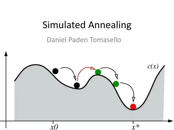
So in the first place...what is simulated annealing? • According to wikipedia : “A probabilistic metaheuristic for the optimization problem of locating a good approximaiton to the global optimum of a given function in a large search space” • When you need some “good enough” solution • For problems with many local minima • Often used in very large discrete spaces
Annealing • Originally a blacksmithing technique in which you cool down the metal slowly • Used to improve ductility and allow further manipulation/shaping
Some notions of Stat.Mechs So why is that, physically? • Gibbs free energy • Each configuration is possible, but weighted by a boltzmann factor : • Slow cooling : minimum energy configuration • Fast cooling (quenching) : polycristals,
Some notions of Stat.Mechs Example : Spin of a chain of atoms • Possible states : Si = ±1 • Energy of a link : Eij = JSiSj • Maximum/minimum is ±NJ (for N the chain length) • Distribution of energy states given by boltzmann... • Thus at low temperature : all spins align • But is low temperature enough in physical systems?
How SA works... So basically, we are going to do the same thing with functions! • Start by “baking” up the system (high randomization) • Gradually cool down (structure appears) • Enjoy
The Method (with a big M) Element 1 : Description Exact description of the state of the possible configurations Example : the N-Queens problems Possible representation of the system : a vector In this case, {7,5,2,6,3,7,8,4}
The Method Element 2 : Generator of random changes Some kind of way of evolving the system → allowed moves Requires some insight of the way the system is working In this case : select an attacked queen, and move it to some random spot on the same row
The Method Element 3 : Objective function Basically, the function to optimize; might not always be obvious in discrete systems Analog of energy In this case :
The Method Element 4 : Acceptance probability function The probability of taking the step to the new proposed state Generally : • Formally, some function of the form P(E1,E2,T)
The Method Element 5 : Annealing schedule The specific way in which the temperature is going to flow from high to low Will make the difference between a working algorithm/PAIN Meaning of fast/slow cooling and hot/cold highly case-specific Here : T(n) = 100/n
The Method Further considerations • Resets • Specific heat calculation
Combinatorial minimization • Type of minimization where there is no continuous spectrum of values for the energy function equivalent • Can be hard to conceptualize : • Energy function might not be obvious • The most efficient way to get to neighbour states might also not be obvious, and can require a lot of thinking
Combinatorial minimization The Traveling Salesman Problem • Given a list of cities and the distances between each pair of cities, what is the shortest possible route that visits each city exactly once and returns to the origin city? • This is harder than it looks... • Possible solutions grow as O(n!) • Exact computation of solutions grows as O(exp(n))
Combinatorial minimization The Traveling Salesman Problem : Description • A state can be defined as one distinct possible route passing through all cities • Supposing N cities, a vector of length N can specify the order in which to visit them For example with N=6 : {C1, C4, C2, C3,C6, C5} • Must also specify the position of each city Supposing 2D, thats {xi,yi}
Combinatorial minimization The Traveling Salesman Problem : Generator This one can be a bit tricky... • Take two random cities and swap them • Take two consecutive cities and swap them • Take two non-consecutive cities and swap the whole segment between them
Combinatorial minimization The Traveling Salesman Problem : Objective function Pretty simple. We have the position of each city... This is basically the total distance function. Note : point N is the same as first point
Combinatorial minimization The Traveling Salesman Problem : Annealing schedule This is the part that requires experimentation... In the literature, some considerations : • If the square in which the cities are located has a side of N1/2, then temperatures above N1/2 can be considered hot, and temperatures below 1 are cold; • Every 100 steps OR 10 successful reconfigurations, multiply temperature by 0.9 • Could also be some continuous equivalent...
Combinatorial minimization The Traveling Salesman Problem : Some results T = 1.2 T = 0.8
Combinatorial minimization The Traveling Salesman Problem : Some results T = 0.4 T = 0.0
Combinatorial minimization The Traveling Salesman Problem : Some results Constraints :
Continuous minimization Kinda simpler, at least conceptually : • Description : System state is some point x • Generator : x+dx where dx is generated somewhat randomly This is where we actually have some room to mess around... the way dx is specified is entirely up to us • Function : Function. • Annealing schedule : Should be gradual once again, but strongly depends on the function being minimized.
Continuous minimization An example of implementation (NR Webnote 1) Return of the AMOEBA! 1. 3. 2. 4.
Continuous minimization An example of implementation • Except here’s a twist... • A positive thermal fluctuation is added to all of the old values of the simplex • Another fluctuation is subtracted from the value of the proposal point • Thus the new point is favored over old points for high temperatures
Applications • Lenses : Merit function depends on a lot of factors : curvature radii, densities, thickness, etc. • Placement problems : When you have to place a lot of stuff in a very limited space... how do you arrange them optimally? Used in logic boards, processors
Conclusion • Simulated annealing is cool (after some time) • Allows to research a large parameter space without getting bogged down in local minima • Very useful for discrete, combinatory problems for which there are not a lot of algorithms (since most are gradient based) • Questions?
Simulated annealing Round 2 !
Revisiting... • Specific heat calculation • Parameter spaces & objective functions • Simulated Annealing vs MCMC
Specific heat calculation Reminder : we can define an equivalent to specific heat for a given problem through the energy (objective) function : But how many steps do we need to get some acceptable value for Cv? Answer : it basically depends on E, and more specifically on the variance of Cv.
Specific heat calculation Thus this will be case-specific. All points considered to get <E> and <E2> are taken at the same temperature; thus the annealing schedule should be arranged with blocks of constant temperature Cv‘s variance is usually pretty large, so we need a lot of data. As an example, for a function : ... at least 10k points/block.
Parameter spaces & objective functions Generally speaking... • Parameter space : • Figure out what parameters you need to describe a state exactly; these can be integers, real numbers, or whatever else you need • Write it out in vector form (or possibly even matrix form), ie. [P1 , P2 , ... Pn] • The set of all possible vectors (varying the parameters that you defined in 1) is your parameter space • Objective function : • Write out the objective function in terms of the previously defined parameters
Parameter spaces & objective functions The traveling salesman problem • Parameter space : • Set of all possible ways to fill visit all cities once. We have N cities, and we need 3 infos for each : xi position, yi position, and rank at which the city will be visited Ri • Objective function :
Parameter spaces & objective functions The knapsack problem
Parameter spaces & objective functions The knapsack problem • Parameter space : • Set of all possible ways to fill the sack without busting. Suppose we have N types of objects; we need 3 infos for each object : the number ni of objects of that type in the sack, the weight mi, and some value Vi • Objective function :
Parameter spaces & objective functions The spanning tree problem Given a weighted graph (set of vertices and weighted links between these), what is the minimum value subgraph that connects all vertices?
Parameter spaces & objective functions The spanning tree problem • Parameter space : Set of all the M links, to which we attribute an activation value µi= 0,1 and weight xi For N the number of vertices, there are N – 1 degrees of freedom
Parameter spaces & objective functions The spanning tree problem • Objective function : where µi = 1 or 0 (active/inactive link)
Parameter spaces & objective functions The N-queens problem • Parameter space : • Set of all possible ways to place the N queens, supposing there is one per row. For each queen we need only the column position xi : • Objective function :
Parameter spaces & objective functions The N-queens problem
Simulated Annealing vs MCMC Needs of each method : Continuous case SA MCMC • Generator function : some way to generate a proposal point x+dx • Acceptance function (almost always) : • Annealing schedule (how, specifically, will the temperature decrease) • Usually stops after a set number of steps (has no memory of the chain, usually) • Generator function : some way to generate a proposal point x+dx • Acceptance function (commonly) : • Number of chains, starting points, possibly with different temperatures • Usually stops either after a set number of steps or when some condition of minimal error is fulfilled in the variance of the chain (requires keeping the chain in memory!)
Simulated Annealing vs MCMC Needs of each method : Combinatorial case SA MCMC • Generator function : some way to generate a proposal neighbour state • Acceptance function (almost always) : • Annealing schedule (how, specifically, will the temperature decrease) • Usually stops after a set number of steps (has no memory of the chain, usually) • Generator function : some way to generate a proposal neighbour state • Acceptance function (commonly) : • Number of chains, starting points, possibly with different temperatures • Usually stops either after a set number of steps or when some condition of minimal error is fulfilled in the variance of the chain (requires keeping the chain in memory!)
Simulated Annealing vs MCMC Some more considerations... • The choice of method is highly case dependant. • Continuous : MCMCs should be able to handle most cases; SA only to be used for particularly badly behaved objective functions • Combinatorial : MCMCs can work... but most objective functions in combinatorial problems tend to have a lot of very deep minima, so SA is usually best • SA is more demanding computationally, but can search a wider parameter space • MCMCs can easily be parallelized (more chains)


