Download

1 / 53
530 likes | 738 Vues
Applications of HMMs. Yves Moreau 2003-2004. Overview. Profile HMMs Estimation Database search Alignment Gene finding Elements of gene prediction Prokaryotes vs. eukaryotes Gene prediction by homology GENSCAN. GGWWRGdy.ggkkqLWFPSNYV IGWLNGynettgerGDFPGTYV PNWWEGql..nnrrGIFPSNYV

E N D
Applications of HMMs Yves Moreau 2003-2004
Overview • Profile HMMs • Estimation • Database search • Alignment • Gene finding • Elements of gene prediction • Prokaryotes vs. eukaryotes • Gene prediction by homology • GENSCAN
GGWWRGdy.ggkkqLWFPSNYV IGWLNGynettgerGDFPGTYV PNWWEGql..nnrrGIFPSNYV DEWWQArr..deqiGIVPSK-- GEWWKAqs..tgqeGFIPFNFV GDWWLArs..sgqtGYIPSNYV GDWWDAel..kgrrGKVPSNYL -DWWEArslssghrGYVPSNYV GDWWYArslitnseGYIPSTYV GEWWKArslatrkeGYIPSNYV GDWWLArslvtgreGYVPSNFV GEWWKAkslsskreGFIPSNYV GEWCEAgt.kngq.GWVPSNYI SDWWRVvnlttrqeGLIPLNFV LPWWRArd.kngqeGYIPSNYI RDWWEFrsktvytpGYYESGYV EHWWKVkd.algnvGYIPSNYV IHWWRVqd.rngheGYVPSSYL KDWWKVev..ndrqGFVPAAYV Profile HMM • Hidden Markov model for the modeling of protein families and for multiple alignment • Example • Part of the alignment of the SH3 domain • Two conserved regions separated by a variable region
Bgn End Profile HMMs • Hidden Markov Models for multiple alignments • Match, insert, and delete states Deletion Insertion Match
Silent deletion states • Deletions could be modeled by shortcut jumps between states • Problem: number of transitions grows quadratically • Other solution: use parallel states that do not produce any symbol (silent state)
GGWWRGdy.ggkkqLWFPSNYV IGWLNGynettgerGDFPGTYV PNWWEGql..nnrrGIFPSNYV DEWWQArr..deqiGIVPSK-- GEWWKAqs..tgqeGFIPFNFV GDWWLArs..sgqtGYIPSNYV GDWWDAel..kgrrGKVPSNYL -DWWEArslssghrGYVPSNYV GDWWYArslitnseGYIPSTYV GEWWKArslatrkeGYIPSNYV GDWWLArslvtgreGYVPSNFV GEWWKAkslsskreGFIPSNYV GEWCEAgt.kngq.GWVPSNYI SDWWRVvnlttrqeGLIPLNFV LPWWRArd.kngqeGYIPSNYI RDWWEFrsktvytpGYYESGYV EHWWKVkd.algnvGYIPSNYV IHWWRVqd.rngheGYVPSSYL KDWWKVev..ndrqGFVPAAYV Corresponding profile HMM .85 HMM from multiple alignment Multiple alignment (+ conserved columns) Parameter estimation = estimation with known paths
.33 .85 New profile HMM Pseudocounts • Zero probabilities in HMM causes the rejection of sequences containing previously unseen residues • To avoid this problem, add pseudocounts (add extra counts as if prior data was available)
Database search with profile HMM • The estimated model can be used to detect new members of the protein family in a sequence database (more sensitive than PSI-BLAST) • For each sequence in the database, we compute P(x, p* | M) (Viterbi) or P(x | M) (forward-backward) • In practice we work with log-odds (w.r.t. the random model P(x | R))
Alignment to profile HMM • Through Viterbi (search for the best alignment path), we can align sequences w.r.t a profile HMM • Training sequences • Database matches
Multiple alignment with profile HMM • If the sequences are not aligned, it is possible to train a profile HMM to align them • Initialization: choose the length of the profile HMM • Length of profile HMM is number of match states sequence length • Training: estimate the model via Viterbi training or Baum-Welch training • Heuristics to avoid local minimas • Multiple alignment: use Viterbi decoding to align sequences
Extensions • More sophisticated pseudocounts are possible • Dirichlet mixtures • Different types of local alignments can be done with HMMs • Methods are available to weigh sequences in function of evolutionary distances
Protein families • PFAM • http://www.sanger.ac.uk/Software/Pfam/search.shtml • Collection of protein families and protein domains • Provides multiple alignment of the protein families for the domains • Provides the domain organization of proteins • Provides profile HMMs of the domains
Software for profile HMMs • SAM: University of California Santa Cruz • http://www.cse.ucsc.edu/research/compbio/sam.html • Web service: http://www.cse.ucsc.edu/research/compbio/HMM-apps/HMM-applications.html (takes time) • Hmmer (‘hammer’): Washington University, St. Louis • http://genome.wustl.edu/eddy/hmmer.html
Overview • Elements of gene prediction • Prokaryotes vs. eukaryotes • Gene prediction by homology • GENSCAN
Evidence for gene prediction • Sources of evidence (positive and negative) • Sequence similarity to known genes (e.g., found by BLASTX) • Statistical measure of codon bias • Template matches to functional sites (e.g., splice site) • Similarity to features not likely to overlap coding sequence (e.g., Alu repeats) • The structure must respect the biological grammar (promoter, exon, intro, ...)
Search by signal vs. search by content • Search by signal • Detect short signals in the genome • E.g., splice site, signal peptide, glycosylation site • Neural networks can be useful here • Search by content • Detect extended regions in the genome • e.g., coding regions, CpG islands • Hidden Markov Models are useful here • Gene finding algorithms combine both
Probabilistic prediction vs. homology • Hidden Markov Models can be used to predict genes • Homology to a known gene is also a strong method for detecting genes • More and more gene prediction packages combine both approaches
Transcription start and stop -35 region TATA box Translation start and stop Open Reading Frames Shine-Delgarno motif Start ATG/GTG Stop TAA/TAG/TGA Stem-loops Operon Signals in prokaryotes
Problems for prokaryotes • Short genes are hard to detect • Operons • Overlapping genes
Transcription Promotor/enhancer/silencer TATA box Introns/exons Donor/acceptor/branch PolyA Repeats Alu, satellites CpG islands Cap/CCAAT&GC boxes Translation 5’ and 3’ UTR Kozak consensus Start ATG Stop TAA/TAG/TGA Signals in eukaryotes
Open reading frames • Translate the sequence into the six possible reading frames • Check for start and stop codons
Codon bias • In coding sequences, genomes have specific biases for the use of codons encoding the same amino acid
Coding potential • Most coding potentials are based on analysis of codon usage • The HMMs keeps track of some kind of average coding potential around each position • The increase and decrease of the coding potential will “push” the HMM in and out of the exons
Promoter region • Promoter region contains the elements that control the expression of the gene • Prediction of the promoter region (e.g., prediction of the TATA-box) is difficult
Intron-exon splicing • Consensus • 5’ Donor • (A,C)AG/GT(A,G)AGT • 3’ Acceptor • TTTTTNCAG/GCCCCC • Branch • CT(G,A)A(C,T) • Neural networks can predict splice sites; they can detect complex correlation between positions in a functional site
Gene prediction by homology • Coding regions evolve more slowly than noncoding ones (conserved by natural selection because of their functional role) • Not only the protein sequence but also the gene structure can be conserved • Use standard homology methods • Gene syntax must be respected
Procrustes • Find potentially related with BLASTX (= model sequences) • Find all possible blocks (exons) on the basis of acceptor/donor location • Look which blocks can be aligned with model sequences • Look for best alignment of blocks with the query sequence
Gene prediction by homology • Advantages • Recognition of short exons and atypical exons • Correct assembly of complex genes (> 10 exons) • Disadvantages • Genes without known homologs are missed • Good homologs necessary for the prediction of the gene structure • Very sensitive to sequencing errors
GENSCAN • GENSCAN was used for the annotation of the human genome in the Human Genome Project • Gene prediction with Hidden Semi-Markov Models • Different models in function of GC-content (<43% G+C, 43-50%, 50-57%, >57%)
Signal: human splice site • 5’ splice site • 3’ splice site
Example • Nodes of HSMM • Position-weight matrix (signal) • Higher-order position-weight matrix • HMM (content)
Training of HSMM Viterbi algorithm for HSMMs Viterbi algorithm
Gene structure prediction • Current performance on exon prediction is acceptable • However, grouping the correct exons into the genes is still problematic • In many cases, a significant proportion of the predicted genes will not be correct
CpG islands • In mammalians, CpG islands have higher G+C and CG dinucleotide content than the rest of the DNA • CpG islands arise in active regions where no deactivation by methylation takes place (CG dinucleotides in methylated regions disappear by deamination) • CpG islands may be used as gene markers in mammalians
Repeats • Repeats make up a large part of the human genome • Alu repeats • Long Interspersed Elements (LINEs) • Short Interspersed Elements (SINEs) • Important to mask repeats when searching for genes
Polyadenylation signal • Polyadenylation (cleavage of pre-mRNA 3' end and synthesis of poly-(A) tract) is a very important early step of pre-mRNA processing • The most well-known signal involved in this process is AATAAA, located 15-20 nucleotides upstream from the poly-(A) site (site of cleavage) • Real AATAAA signals can differ from AATAAA consensus sequence. The most frequent natural variant, ATTAAA, is nearly as active as the canonical sequence.