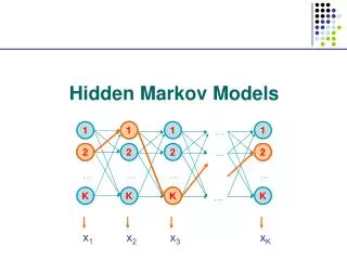
Hidden Markov Models (HMMs)
Hidden Markov Models (HMMs). (Lecture for CS410 Text Information Systems) April 24, 2009 ChengXiang Zhai Department of Computer Science University of Illinois, Urbana-Champaign. Modeling a Multi-Topic Document. A document with 2 subtopics, thus 2 types of vocabulary. …

Hidden Markov Models (HMMs)
E N D
Presentation Transcript
Hidden Markov Models (HMMs) (Lecture for CS410 Text Information Systems) April 24, 2009 ChengXiang Zhai Department of Computer Science University of Illinois, Urbana-Champaign
Modeling a Multi-Topic Document A document with 2 subtopics, thus 2 types of vocabulary … text mining passage food nutrition passage text mining passage text mining passage food nutrition passage … How do we model such a document? How do we “generate” such a document? How do we estimate our model? We’ve already seen one solution – unigram mixture model + EM This lecture is about another (better) solution – HMM + EM
Simple Unigram Mixture Model … text 0.2 mining 0.1 assocation 0.01 clustering 0.02 … food 0.00001 … =0.7 Model/topic 1 p(w|1) … food 0.25 nutrition 0.1 healthy 0.05 diet 0.02 … 1-=0.3 Model/topic 2 p(w|2) p(w|1 2) = p(w|1)+(1- )p(w|2)
Topic 1= text mining p(w|1) Topic 1= text mining p(w|1) Topic 2= health p(w|2) Deficiency of the Simple Mixture Model • Adjacent words are sampled independently • Cannot ensure passage cohesion • Cannot capture the dependency between neighboring words We apply the text mining algorithm to the nutrition data to find patterns … Solution=?
The Hidden Markov Model Solution • Basic idea: • Make the choice of model for a word depend on the choice of model for the previous word • Thus we model both the choice of model (“state”) and the words (“observations”) O: We apply the text mining algorithm to the nutrition data to find patterns … S1: 1 1 1 1 1 1 1 1 1 1 1 1 1 …… O: We apply the text mining algorithm to the nutrition data to find patterns … S2: 1 1 1 1 1 1 1 1 2 1 1 1 1 P(O,S1) > p(O,S2)?
O:…......... ….. We apply the text mining … patterns. ……………… S2: BB...BB T T T T T …. T BB….. BBBB Another Example: Passage Retrieval • Strategy I: Build passage index • Need pre-processing • Query independent boundaries • Efficient • Strategy II: Extract relevant passages dynamically • No pre-processing • Dynamically decide the boundaries • Slow Relevant Passages (“T”) Background text (“B”) O: We apply the text mining algorithm to thenutrition data to find patterns … S1: B T B T T T B B T T B T T
0.8 0.8 0.5 0.5 0.2 0.2 B B T T 0.5 0.5 P(w|T) P(w|T) A Simple HMM for Recognizing Relevant Passages Parameters Initial state prob: p(B)= 0.5; p(T)=0.5 State transition prob: p(BB)=0.8 p(BT)=0.2 p(TB)=0.5 p(TT)=0.5 Output prob: P(“the”|B) = 0.2 … P(“text”|T) = 0.1 … P(B)=0.5 P(T)=0.5 P(w|B) P(w|B) the 0.2 a 0.1 we 0.01 to 0.02 … text 0.0001 mining 0.00005 … … text =0.125 mining = 0.1 association =0.1 clustering = 0.05 … Topic Background
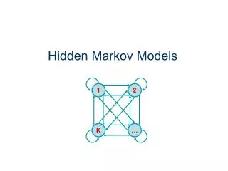
A General Definition of HMM Initial state probability: N states State transition probability: M symbols Output probability:
B T 0.2 0.5 0.5 0.5 0.8 0.2 0.5 B T T T B B T B 0.5 0.2 0.125 0.1 0.1 0.02 0.1 0.05 0.0001 How to “Generate” Text? P(w|B) P(w|T) 0.8 0.5 the 0.2 a 0.1 we 0.01 is 0.02 … method 0.0001 mining 0.00005 … 0.2 … text =0.125 mining = 0.1 algorithm =0.1 clustering = 0.05 … 0.5 P(B)=0.5 P(T)=0.5 the text mining algorithm is a clustering method P(BTT…,”the text mining…”)=p(B)p(the|B) p(T|B)p(text|T) p(T|T)p(mining|T)… = 0.5*0.2 * 0.2*0.125 * 0.5*0.1…
HMM as a Probabilistic Model Time/Index: t1 t2 t3 t4 … Data: o1 o2 o3 o4 … Sequential data Random variables/ process Observation variable: O1 O2 O3 O4 … Hidden state variable: S1 S2 S3 S4 … State transition prob: Probability of observations with known state transitions: Output prob. Joint probability (complete likelihood): Init state distr. Probability of observations (incomplete likelihood): State trans. prob.
Three Problems 1. Decoding – finding the most likely path Given: model, parameters, observations (data) Find: most likely states sequence (path) 2. Evaluation – computing observation likelihood Given: model, parameters, observations (data) Find: the likelihood to generate the data
Three Problems (cont.) 3. Training – estimating parameters • Supervised Given: model structure, labeled data( data+states sequence) Find: parameter values • Unsupervised Given: model structure, data (unlabeled) Find: parameter values
Problem I: Decoding/ParsingFinding the most likely path This is the most common way of using an HMM (e.g., extraction, structure analysis)…
B T ? ? ? ? ? ? ? ? ? ? ? ? ? ? ? ? ? ? ? ? ? ? ? ? What’s the most likely path? P(w|B) P(w|T) 0.8 0.5 the 0.2 a 0.1 we 0.01 is 0.02 … method 0.0001 mining 0.00005 … 0.2 … text =0.125 mining = 0.1 algorithm =0.1 clustering = 0.05 … 0.5 P(B)=0.5 P(T)=0.5 the text mining algorithm is a clustering method
B T Viterbi Algorithm: An Example P(w|B) 0.8 P(w|T) 0.5 the 0.2 a 0.1 we 0.01 … algorithm 0.0001 mining 0.005 text 0.001 … the 0.05 text =0.125 mining = 0.1 algorithm =0.1 clustering = 0.05 0.2 0.5 P(T)=0.5 P(B)=0.5 t = 1 2 3 4 … the text mining algorithm … 0.5 0.8 0.8 0.8 B B B B 0.2 0.2 0.2 0.5 0.5 0.5 0.5 0.5 T 0.5 T 0.5 T T VP(B): 0.5*0.2 (B) 0.5*0.2*0.8*0.001(BB) … *0.5*0.005 (BTB)…*0.5*0.0001(BTTB) VP(T) 0.5*0.05(T) 0.5*0.2*0.2*0.125(BT) … *0.5*0.1 (BTT) …*0.5*0.1(BTTT) Winning path! 0.5
Viterbi Algorithm Observation: Algorithm: (Dynamic programming) Complexity: O(TN2)
Problem II: EvaluationComputing the data likelihood Another use of an HMM, e.g., as a generative model for classification Also related to Problem III – parameter estimation
Data Likelihood: p(O|) t = 1 2 3 4 … the text mining algorithm … 0.5 0.8 0.8 0.8 B B B B 0.2 0.2 0.2 0.5 0.5 0.5 0.5 0.5 T 0.5 T 0.5 T T In general, enumerate all paths BB… B BT… B TT… T Complexity of a naïve approach? 0.5
The Forward Algorithm … B B B B … T T T T α1
The Forward Algorithm … B B B B … T T T T α1 α2
The Forward Algorithm … B B B B … T T T T α4 α1 α2 α3 Generating o1…ot with ending state si The data likelihood is Complexity: O(TN2)
Forward Algorithm: Example t = 1 2 3 4 … the text mining algorithm … 0.5 0.8 0.8 0.8 B B B B 0.2 0.2 0.2 0.5 0.5 0.5 0.5 0.5 T 0.5 T 0.5 T T 1(B): 0.5*p(“the”|B) 2(B): [1(B)*0.8+ 1(T)*0.5]*p(“text”|B) …… 1(T): 0.5*p(“the”|T) 2(T): [1(B)*0.2+ 1(T)*0.5]*p(“text”|T) …… P(“the text mining algorithm”) = 4(B)+ 4(T)
The Backward Algorithm Observation: Algorithm: (o1…ot already generated) Starting from state si Generating ot+1…oT Complexity: O(TN2) The data likelihood is
Backward Algorithm: Example t = 1 2 3 4 … the text mining algorithm … 0.5 0.8 0.8 0.8 B B B B 0.2 0.2 0.2 0.5 0.5 0.5 0.5 0.5 T 0.5 T 0.5 T T … … 4(B): 1 3(B): 0.8*p(“alg”|B)*4(B)+ 0.2*p(“alg”|T)*4(T) 3(T): 0.5*p(“alg”|B)*4(B)+ 0.5*p(“alg”|T)*4(T) 4(T): 1 P(“the text mining algorithm”) = 1(B)*1(B)+ 1(T)* 1(T) = 2(B)*2(B)+ 2(T)* 2(T)
Problem III: TrainingEstimating Parameters Where do we get the probability values for all parameters? Supervised vs. Unsupervised
1=1/1=1; 2=0/1=0 a11=2/4=0.5; a12=2/4=0.5 a21=1/5=0.2; a22=4/5=0.8 b1(a)=4/4=1.0; b1(b)=0/4=0; b2(a)=1/6=0.167; b2(b)=5/6=0.833 0.5 0.8 0.5 P(s1)=1 P(s2)=0 1 2 0.2 P(a|s1)=1 P(b|s1)=0 P(a|s2)=167 P(b|s2)=0.833 Supervised Training Given: 1. N – the number of states, e.g., 2, (s1 and s2) 2. V – the vocabulary, e.g., V={a,b} 3. O – observations, e.g., O=aaaaabbbbb 4. State transitions, e.g., S=1121122222 Task: Estimate the following parameters 1. 1, 2 2. a11, a12, a22, a21 3. b1(a), b1(b), b2(a), b2(b)
Unsupervised Training Given: 1. N – the number of states, e.g., 2, (s1 and s2) 2. V – the vocabulary, e.g., V={a,b} 3. O – observations, e.g., O=aaaaabbbbb 4. State transitions, e.g., S=1121122222 Task: Estimate the following parameters 1. 1, 2 2. a11, a12, a22, a21 3. b1(a), b1(b), b2(a), b2(b) How could this be possible? Maximum Likelihood:
Intuition O=aaaaabbbbb, P(O,q1|) P(O,qK|) P(O,q2|) q1=1111111111 q2=11111112211 … qK=2222222222 New ’ Computation of P(O,qk|) is expensive …
Baum-Welch Algorithm Basic “counters”: Being at state si at time t Being at state si at time t and at state sj at time t+1 Computation of counters: Complexity: O(N2)
Baum-Welch Algorithm (cont.) Updating formulas: Overall complexity for each iteration: O(TN2)
What You Should Know • Definition of an HMM • What are the three problems associated with an HMM? • Know how the following algorithms work • Viterbi algorithm • Forward & Backward algorithms • Know the basic idea of the Baum-Welch algorithm
Readings • Read [Rabiner 89] sections I, II, III • Read the “brief note”