Hidden Markov Models: Application in Bioinformatics
300 likes | 409 Vues
This lecture covers the application of Hidden Markov Models (HMMs) in solving the CpG island problem, focusing on methylation in the human genome. The lecture discusses how to identify CpG islands in genomic sequences using Bayesian classifiers and generative models. It also explains how HMMs can be used for modeling sequences and solving problems like Decoding, Evaluation, and Training.

Hidden Markov Models: Application in Bioinformatics
E N D
Presentation Transcript
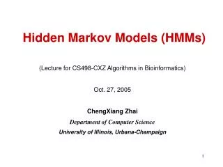
Hidden Markov Models (HMMs) (Lecture for CS498-CXZ Algorithms in Bioinformatics) Oct. 27, 2005 ChengXiang Zhai Department of Computer Science University of Illinois, Urbana-Champaign
Motivation: the CpG island problem • Methylation in human genome • “CG” -> “TG” happens in most place except “start regions” of genes • CpG islands = 100-1,000 bases before a gene starts • Questions • Q1: Given a short stretch of genomic sequence, how would we decide if it comes from a CpG island or not? • Q2: Given a long sequence, how would we find the CpG islands in it?
Answer to Q1: Bayes Classifier Hypothesis space: H={HCpG,HOther} Evidence: X=“ATCGTTC” Prior probability Likelihood of evidence (Generative Model) We need two generative models for sequences: p(X| HCpG), p(X|HOther)
A Simple Model for Sequences:p(X) Probability rule Assume independence Capture some dependence P(x|HCpG) P(A|HCpG)=0.25 P(T|HCpG)=0.25 P(C|HCpG)=0.25 P(G|HCpG)=0.25 P(x|HOther) P(A|HOther)=0.25 P(T|HOther)=0.40 P(C|HOther)=0.10 P(G|HOther)=0.25 X=ATTG Vs. X=ATCG
How can we identify a CpG island in a long sequence? Idea 1: Test each window of a fixed number of nucleitides Idea2: Classify the whole sequence Class label S1: OOOO………….……O Class label S2: OOOO…………. OCC … Class label Si: OOOO…OCC..CO…O … Class label SN: CCCC……………….CC S*=argmaxS P(S|X) = argmaxS P(S,X) S*=OOOO…OCC..CO…O CpG Answer to Q2: Hidden Markov Model X=ATTGATGCAAAAGGGGGATCGGGCGATATAAAATTTG Other CpG Island Other
B I A simple HMM 0.8 0.8 Parameters Initial state prob: p(B)= 0.5; p(I)=0.5 State transition prob: p(BB)=0.8 p(BI)=0.2 p(IB)=0.5 p(II)=0.5 Output prob: P(a|B) = 0.25, … p(c|B)=0.10 … P(c|I) = 0.25 … 0.5 0.5 P(B)=0.5 P(I)=0.5 0.2 0.2 P(x|B) P(x|I) 0.5 0.5 P(x|HCpG)=p(x|I) P(a|I)=0.25 P(t|I)=0.25 P(c|I)=0.25 P(g|I)=0.25 P(x|HOther)=p(x|B) P(a|B)=0.25 P(t|B)=0.40 P(c|B)=0.10 P(g|B)=0.25
A General Definition of HMM Initial state probability: N states State transition probability: M symbols Output probability:
B I How to “Generate” a Sequence? P(x|B) P(x|I) 0.8 0.5 P(a|B)=0.25 P(t|B)=0.40 P(c|B)=0.10 P(g|B)=0.25 P(a|I)=0.25 P(t|I)=0.25 P(c|I)=0.25 P(g|I)=0.25 0.2 model 0.5 P(B)=0.5 P(I)=0.5 a c g t t … Sequence B I I I B B I B states I I I B B I I B … … Given a model, follow a path to generate the observations.
B I How to “Generate” a Sequence? P(x|B) P(x|I) 0.8 0.5 P(a|B)=0.25 P(t|B)=0.40 P(c|B)=0.10 P(g|B)=0.25 P(a|I)=0.25 P(t|I)=0.25 P(c|I)=0.25 P(g|I)=0.25 0.2 model 0.5 P(B)=0.5 P(I)=0.5 a c g t t … Sequence 0.2 0.5 0.5 0.5 B I I I B 0.5 0.25 0.25 0.25 0.25 0.4 t a c g t P(“BIIIB”, “acgtt”)=p(B)p(a|B) p(I|B)p(c|I)p(I|I)p(g|I)p(I|I)p(t|I)p(B|I)p(t|B)
HMM as a Probabilistic Model Time/Index: t1 t2 t3 t4 … Data: o1 o2 o3 o4 … Sequential data Random variables/ process Observation variable: O1 O2 O3 O4 … Hidden state variable: S1 S2 S3 S4 … State transition prob: Probability of observations with known state transitions: Output prob. Joint probability (complete likelihood): Init state distr. Probability of observations (incomplete likelihood): State trans. prob.
Three Problems 1. Decoding – finding the most likely path Given: model, parameters, observations (data) Compute: most likely states sequence 2. Evaluation – computing observation likelihood Given: model, parameters, observations (data) Compute: the likelihood to generate the observed data
Three Problems (cont.) 3 Training – estimating parameters • Supervised Given: model architecture, labeled data ( data+state sequence) • Unsupervised Given : model architecture, unlabeled data Maximum Likelihood
Problem I: Decoding/ParsingFinding the most likely path You can think of this as classification with all the paths as class labels…
B I ? ? ? ? ? ? ? ? ? ? ? ? ? ? ? ? ? ? ? ? ? ? ? ? What’s the most likely path? P(x|B) P(x|I) 0.8 P(a|B)=0.25 P(t|B)=0.40 P(c|B)=0.10 P(g|B)=0.25 0.5 P(a|I)=0.25 P(t|I)=0.25 P(c|I)=0.25 P(g|I)=0.25 0.2 0.5 P(B)=0.5 P(I)=0.5 a c g t t a t g
B I Viterbi Algorithm: An Example 0.8 0.5 P(x|B) P(a|B)=0.251 P(t|B)=0.40 P(c|B)=0.098 P(g|B)=0.251 P(x|I) 0.2 P(a|I)=0.25 P(t|I)=0.25 P(c|I)=0.25 P(g|I)=0.25 0.5 P(B)=0.5 P(I)=0.5 t = 1 2 3 4 … a c g t … 0.5 0.8 0.8 0.8 B B B B 0.2 0.2 0.2 0.5 0.5 0.5 0.5 0.5 I 0.5 I 0.5 I I VP(B): 0.5*0.251 (B) 0.5*0.251*0.8*0.098(BB) … VP(I) 0.5*0.25(I) 0.5*0.25*0.5*0.25(II) … Remember the best paths so far 0.5
Viterbi Algorithm Observation: Algorithm: (Dynamic programming) Complexity: O(TN2)
Problem II: EvaluationComputing the data likelihood Another use of an HMM, e.g., as a generative model for discrimination Also related to Problem III – parameter estimation
Data Likelihood: p(O|) t = 1 2 3 4 … a c g t … 0.5 0.8 0.8 0.8 B B B B 0.2 0.2 0.2 0.5 0.5 0.5 0.5 0.5 I 0.5 I 0.5 I I All HMM parameters In general, Complexity of a naïve approach? 0.5
The Forward Algorithm Observation: Algorithm: Generating o1…ot with ending state si The data likelihood is Complexity: O(TN2)
Forward Algorithm: Example t = 1 2 3 4 … a c g t … 0.5 0.8 0.8 0.8 B B B B 0.2 0.2 0.2 0.5 0.5 0.5 0.5 0.5 I 0.5 I 0.5 I I 1(B): 0.5*p(“a”|B) 2(B): [1(B)*0.8+ 1(I)*0.5]*p(“c”|B) …… 1(I): 0.5*p(“a”|I) 2(I): [1(B)*0.2+ 1(I)*0.5]*p(“c”|I) …… P(“a c g t”) = 4(B)+ 4(I)
The Backward Algorithm Observation: Algorithm: (o1…ot already generated) Starting from state si Generating ot+1…oT Complexity: O(TN2) The data likelihood is
Backward Algorithm: Example t = 1 2 3 4 … a c g t … 0.5 0.8 0.8 0.8 B B B B 0.2 0.2 0.2 0.5 0.5 0.5 0.5 0.5 I 0.5 I 0.5 I I … … 4(B): 1 3(B): 0.8*p(“t”|B)*4(B)+ 0.2*p(“t”|I)*4(I) 3(I): 0.5*p(“t”|B)*4(B)+ 0.5*p(“t”|T)*4(I) 4(I): 1 P(“a c g t”) = 1(B)*1(B)+ 1(I)* 1(I) = 2(B)*2(B)+ 2(I)* 2(I)
Problem III: TrainingEstimating Parameters Where do we get the probability values for all parameters? Supervised vs. Unsupervised
Supervised Training Given: 1. N – the number of states, e.g., 2, (s1 and s2) 2. V – the vocabulary, e.g., V={a,b} 3. O – observations, e.g., O=aaaaabbbbb 4. State transitions, e.g., S=1121122222 Task: Estimate the following parameters 1. 1, 2 2. a11, a12,a22,a21 3. b1(a), b1(b), b2(a), b2(b) 1=1/1=1; 2=0/1=0 a11=2/4=0.5; a12=2/4=0.5 a21=1/5=0.2; a22=4/5=0.8 b1(a)=4/4=1.0; b1(b)=0/4=0; b2(a)=1/6=0.167; b2(b)=5/6=0.833 0.5 0.8 0.5 P(s1)=1 P(s2)=0 1 2 0.2 P(a|s1)=1 P(b|s1)=0 P(a|s2)=167 P(b|s2)=0.833
Unsupervised Training Given: 1. N – the number of states, e.g., 2, (s1 and s2) 2. V – the vocabulary, e.g., V={a,b} 3. O – observations, e.g., O=aaaaabbbbb 4. State transitions, e.g., S=1121122222 Task: Estimate the following parameters 1. 1, 2 2. a11, a12,a22,a21 3. b1(a), b1(b), b2(a), b2(b) How could this be possible? Maximum Likelihood:
Intuition O=aaaaabbbbb, P(O,q1|) P(O,qK|) P(O,q2|) q1=1111111111 q2=11111112211 … qK=2222222222 New ’ Computation of P(O,qk|) is expensive …
Baum-Welch Algorithm Basic “counters”: Being at state si at time t Being at state si at time t and at state sj at time t+1 Computation of counters: Complexity: O(N2)
Baum-Welch Algorithm (cont.) Updating formulas: Overall complexity for each iteration: O(TN2)
What You Should Know • Definition of an HMM and parameters of an HMM • Viterbi Algorithm • Forward/Backward algorithms • Estimate parameters of an HMM in a supervised way