Hidden Markov Models

1. Hidden Markov Models Bonnie Dorr Christof Monz CMSC 723: Introduction to Computational Linguistics Lecture 5 October 6, 2004

2. Hidden Markov Model (HMM) • HMMs allow you to estimate probabilities of unobserved events • Given plain text, which underlying parameters generated the surface • E.g., in speech recognition, the observed data is the acoustic signal and the words are the hidden parameters

3. HMMs and their Usage • HMMs are very common in Computational Linguistics: • Speech recognition (observed: acoustic signal, hidden: words) • Handwriting recognition (observed: image, hidden: words) • Part-of-speech tagging (observed: words, hidden: part-of-speech tags) • Machine translation (observed: foreign words, hidden: words in target language)

4. Noisy Channel Model • In speech recognition you observe an acoustic signal (A=a1,…,an) and you want to determine the most likely sequence of words (W=w1,…,wn): P(W | A) • Problem: A and W are too specific for reliable counts on observed data, and are very unlikely to occur in unseen data

5. Noisy Channel Model • Assume that the acoustic signal (A) is already segmented wrt word boundaries • P(W | A) could be computed as • Problem: Finding the most likely word corresponding to a acoustic representation depends on the context • E.g., /'pre-z&ns / could mean “presents” or “presence” depending on the context

6. Noisy Channel Model • Given a candidate sequence W we need to compute P(W) and combine it with P(W | A) • Applying Bayes’ rule: • The denominator P(A) can be dropped, because it is constant for all W

7. Noisy Channel in a Picture

8. Decoding The decoder combines evidence from • The likelihood: P(A | W) This can be approximated as: • The prior: P(W) This can be approximated as:

9. Search Space • Given a word-segmented acoustic sequence list all candidates • Compute the most likely path

10. Markov Assumption • The Markov assumption states that probability of the occurrence of word wi at time t depends only on occurrence of word wi-1 at time t-1 • Chain rule: • Markov assumption:

11. The Trellis

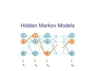
12. Parameters of an HMM • States: A set of states S=s1,…,sn • Transition probabilities: A= a1,1,a1,2,…,an,n Each ai,j represents the probability of transitioning from state si to sj. • Emission probabilities: A set B of functions of the form bi(ot) which is the probability of observation ot being emitted by si • Initial state distribution: is the probability that si is a start state

13. The Three Basic HMM Problems • Problem 1 (Evaluation): Given the observation sequence O=o1,…,oT and an HMM model , how do we compute the probability of O given the model? • Problem 2 (Decoding): Given the observation sequence O=o1,…,oT and an HMM model , how do we find the state sequence that best explains the observations?

14. The Three Basic HMM Problems • Problem 3 (Learning): How do we adjust the model parameters , to maximize ?

15. Problem 1: Probability of an Observation Sequence • What is ? • The probability of a observation sequence is the sum of the probabilities of all possible state sequences in the HMM. • Naïve computation is very expensive. Given T observations and N states, there are NT possible state sequences. • Even small HMMs, e.g. T=10 and N=10, contain 10 billion different paths • Solution to this and problem 2 is to use dynamic programming

16. Forward Probabilities • What is the probability that, given an HMM , at time t the state is i and the partial observation o1 … ot has been generated?

17. Forward Probabilities

18. Forward Algorithm • Initialization: • Induction: • Termination:

19. Forward Algorithm Complexity • In the naïve approach to solving problem 1 it takes on the order of 2T*NT computations • The forward algorithm takes on the order of N2T computations

20. Backward Probabilities • Analogous to the forward probability, just in the other direction • What is the probability that given an HMM and given the state at time t is i, the partial observation ot+1 … oT is generated?

21. Backward Probabilities

22. Backward Algorithm • Initialization: • Induction: • Termination:

23. Problem 2: Decoding • The solution to Problem 1 (Evaluation) gives us the sum of all paths through an HMM efficiently. • For Problem 2, we wan to find the path with the highest probability. • We want to find the state sequence Q=q1…qT, such that

24. Viterbi Algorithm • Similar to computing the forward probabilities, but instead of summing over transitions from incoming states, compute the maximum • Forward: • Viterbi Recursion:

25. Viterbi Algorithm • Initialization: • Induction: • Termination: • Read out path:

26. Problem 3: Learning • Up to now we’ve assumed that we know the underlying model • Often these parameters are estimated on annotated training data, which has two drawbacks: • Annotation is difficult and/or expensive • Training data is different from the current data • We want to maximize the parameters with respect to the current data, i.e., we’re looking for a model , such that

27. Problem 3: Learning • Unfortunately, there is no known way to analytically find a global maximum, i.e., a model , such that • But it is possible to find a local maximum • Given an initial model , we can always find a model , such that

28. Parameter Re-estimation • Use the forward-backward (or Baum-Welch) algorithm, which is a hill-climbing algorithm • Using an initial parameter instantiation, the forward-backward algorithm iteratively re-estimates the parameters and improves the probability that given observation are generated by the new parameters

29. Parameter Re-estimation • Three parameters need to be re-estimated: • Initial state distribution: • Transition probabilities: ai,j • Emission probabilities: bi(ot)

30. Re-estimating Transition Probabilities • What’s the probability of being in state si at time t and going to state sj, given the current model and parameters?

31. Re-estimating Transition Probabilities

32. Re-estimating Transition Probabilities • The intuition behind the re-estimation equation for transition probabilities is • Formally:

33. Re-estimating Transition Probabilities • Defining As the probability of being in state si, given the complete observation O • We can say:

34. Review of Probabilities • Forward probability: The probability of being in state si, given the partial observation o1,…,ot • Backward probability: The probability of being in state si, given the partial observation ot+1,…,oT • Transition probability: The probability of going from state si, to state sj, given the complete observation o1,…,oT • State probability: The probability of being in state si, given the complete observation o1,…,oT

35. Re-estimating Initial State Probabilities • Initial state distribution: is the probability that si is a start state • Re-estimation is easy: • Formally:

36. Re-estimation of Emission Probabilities • Emission probabilities are re-estimated as • Formally: Where Note that here is the Kronecker delta function and is not related to the in the discussion of the Viterbi algorithm!!

37. The Updated Model • Coming from we get to by the following update rules:

38. Expectation Maximization • The forward-backward algorithm is an instance of the more general EM algorithm • The E Step: Compute the forward and backward probabilities for a give model • The M Step: Re-estimate the model parameters