### Understanding Electronic Amplifiers: Principles and Applications ###
This chapter provides a comprehensive overview of electronic amplifiers, a crucial component in signal processing. It starts with the basics of amplification and attenuation, exploring both non-electronic (passive) and electronic (active) amplifiers. Key concepts such as input and output resistance, equivalent circuits, output power, and power gain are discussed, along with their relevance in real-world applications. The effects of loads on amplifier performance and the importance of frequency response and bandwidth are also highlighted. Understanding these principles is essential for designing efficient electronic systems. ###

### Understanding Electronic Amplifiers: Principles and Applications ###
E N D
Presentation Transcript
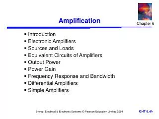
Chapter 6 Amplification • Introduction • Electronic Amplifiers • Sources and Loads • Equivalent Circuits of Amplifiers • Output Power • Power Gain • Frequency Response and Bandwidth • Differential Amplifiers • Simple Amplifiers
6.1 Introduction • Amplification is one of the most common processing functions • Amplification means making things bigger • Attenuation means making things smaller • There are many non-electronic forms of amplification
Non-electronic amplifiers • Levers • Example shown on the right is a force amplifier, but a displacement attenuator • Reversing the input and output would produce a force attenuator but a displacement amplifier • This is an example of a non-inverting amplifier (since the input and output are in the same direction) A lever arrangement
Non-electronic amplifiers • Pulleys • Example shown right is a force amplifier, but a displacement attenuator • This is an example of an inverting amplifier (since the input and output are in opposite directions) but other pulley arrangements can be non-inverting A pulley arrangement
Passive and active amplifiers • levers and pulleys are examples of passive amplifiers since they have no external energy source • in such amplifiers the power delivered at the output must be less than (or equal to) that absorbed at the input • some amplifiers are not passive but are active amplifiers in that they have an external source of power • in such amplifiers the output can deliver more power than is absorbed at the input
Non-electronic active amplifiers • an example is the torque amplifier shown here A torque amplifier
6.2 Electronic Amplifiers • Can be passive (e.g. a transformer) but most are active • We will concentrate on active electronic amplifiers • take power from a power supply • amplification described by gain Circuit symbol
6.3 Sources and Loads • An ideal voltage amplifier would produce an output determined only by the input voltage and its gain • irrespective of the nature of the source and the load • in real amplifiers this is not the case • the output voltage is affected by loading
Modelling the input of an amplifier • the input can often beadequately modelled bya simple resistor • the input resistance
Modelling the output of a circuit • all real voltage sources have an output resistance • for example, a battery can be represented by an ideal voltage source and a series resistance representing its output resistance
Modelling the output of an amplifier • similarly, the output of an amplifier can be modelled by an ideal voltage source and an output resistance • this is an example of a Thévenin equivalent circuit(we will return to such circuits later)
Modelling the gain of an amplifier • can be modelled by a controlled voltage source • the voltage produced by the source is determined by the input voltage to the circuit
6.4 Equivalent Circuits of Amplifiers • Having modelled the input, the output and the gain, we can now model the entire amplifier
The use of an equivalent circuit (see Example 6.1 in the course text): Example: An amplifier has a voltage gain of 10, an input resistance of 1 k and an output resistance of 10 . The amplifier is connected to a sensor that produces a voltage of 2 V and has an output resistance of 100 , and to a load of 50 . What will be the output voltage of the amplifier (that is the voltage across the load resistance)?
We start by constructing an equivalent circuit of the amplifier, the source and the load
The voltage gain of the circuit in the previous example is given by: • note that this is considerably less than the stated gain of the amplifier (which is 10) • this is due to loading effects • the gain of the amplifier in isolation is its unloaded voltage gain
An ideal voltage amplifier would not suffer from loading • it would have Ri = and Ro = 0 • consider the effect on the previous example
If Ri= , then • Therefore • the effects of loading are removed (see Example 6.3)
6.5 Output Power • The output power Po is that dissipated in the load resistor • Power transfer is at a maximum when RL = Ro • maximum power theorem • choosing a load to maximize power transfer is called matching • often voltage gain is more important than power transfer
6.6 Power Gain • Power gain is the ratio of the power supplied to the load to that absorbed at the input • For numerical example see Example 6.5 in set text • Gain often given in decibels
Sample gains expressed in dBs • Using dBs simplifies calculation in cascaded circuits
Power gain is related to voltage gain • If R1 = R2 • This expression is often used even when R1R2 • see Example 6.7 and Example 6.8 in the course text
6.7 Frequency Response and Bandwidth • All real amplifiers have limits to the range of frequencies over which they can be used • The gain of a circuit in its normal operating range is termed its mid-band gain • The gain of all amplifiers falls at high frequencies • characteristic defined by the half-power point • gain falls to 1/2 = 0.707 times the mid-band gain • this occurs at the cut-off frequency • In some amplifiers gain also falls at low frequencies • these are AC coupled amplifiers
(a) shows an AC coupled amplifier • (b) shows the same amplifier – with gain in dBs • (c) shows a DC coupled amplifier – the gain is constant down to DC
The bandwidth is the difference between the upper and lower cut-off frequencies … • … or the difference between the upper-cut-off frequency and zero in a DC coupled amplifier
6.8 Differential Amplifiers • Differential amplifiers have two inputs and amplify the voltage difference between them • inputs are called the non-inverting input (labelled +) and the inverting input (labelled –)
Equivalent circuit of a differential amplifier • one of the commonest forms of differential amplifier is the operational amplifier – discussed in later lectures
6.9 Simple Amplifiers • Operational amplifiers are relatively complex circuits • Amplifiers can also be formed using a ‘control device’ • circuit is similar to a potential divider with one resistor replaced with a ‘control device’ typically a transistor A potential divider A simple amplifier
Key Points • Amplification forms part of most electronic systems • Amplifiers may be active or passive • Equivalent circuits are useful when investigating the interaction between circuits • Amplifier gains are often measured in decibels (dBs) • The gain of all amplifiers falls at high frequencies • The gain of some amplifiers falls at low frequencies • Differential amplifiers take as their input the difference between two input signals • Some amplifiers are very simple in construction