Download
1 / 56
560 likes | 679 Vues
Detection of domestication genes and other loci under selection. Bruce Walsh, jbwalsh@u.arizona.edu University of Arizona Depts. of Ecology & Evolutionary Biology, Molecular & Cellular Biology, Plant Sciences, Animal Sciences, Epidemology & Biostatistics. Search for Genes that experienced

E N D
Detection of domestication genes and other loci under selection Bruce Walsh, jbwalsh@u.arizona.edu University of Arizona Depts. of Ecology & Evolutionary Biology, Molecular & Cellular Biology, Plant Sciences, Animal Sciences, Epidemology & Biostatistics
Search for Genes that experienced artificial (and natural) selection Akin in sprit to testing candidate genes for association or using genome scans to find QTLs. In linkage studies: Use molecular markers to look for marker-trait associations (phenotypes) In tests for selection, use molecular markers to look for patterns of selection (patterns of within- and between-species variation)
Types of Genes that have experienced selection in crop/animal species Domestication genes: Alleles fixed in the course of the initial domestication Diversification/Improvement genes: Alleles fixed in the course of improvement following domestication. Adaptation genes: Alleles in natural populations responding to natural selection on environmental conditions (candidates to transfer into elite germplasms).
The general approaches for using sequence data to search for signs of selection Key: Use of features of variation at a marker locus to test for departures from strict neutrality • Tests based on pattern and amount of within- species polymorphism (departures from neutral predictions). On-going or recent selection • Tests based on polymorphism plus between species divergence. On-going or recent selection • Tests based on phylogenetic comparisons between species. Historical selection (won’t discuss these further)
A quick review of the neutral theory (expected patterns of variation under drift) • Drift and the coalescence process (its about time) • Mutation-drift equilibrium (within-population variation). Function of population size and mutation rate. Expected variation = H = 4Nem • Divergence between populations (between- population variation). Function of time and mutation rate (but not population size), d = 2tm
Mutation-Drift Equilibrium (Single Loci) Drift removes variation, while mutation introduces it. Thus, an equilibrium amount of genetic variance results While alleles change over time, heterozygosity remains roughly constant.
A very powerful way of thinking about drift is the Coalescent Process Instead of following alleles, think in terms of lineages. As a consequence of drift, eventually all current copies of alleles trace back to a single ancestral lineage. Hence, the current lineages coalesce as one moves back in time
From coalescent theory, the expected time back to the MRCA is 2N generations Hence, for two randomly-chosen sequences, the expected number of mutations they differ by is just 2mt = 2m(2N) = 4Nm If 4Nm >> 1, two random sequences will typically differ (and hence be heterozygotes) If 4Nm << 1, two random sequences will typically differ (and hence be homozygotes)
Divergence Between Populations Mutation and drift also generate a between- line variance, i.e., a population divergence As lines separate, the initial heterozygosity is randomly partitioned, creating a between-line variance. More importantly, as new mutations arise in the separated lines, some of these are fixed by drift, and this drives a constant divergence between populations
One average, for a population of size N, 2Nm mutations arise each generation For any of these, their probability of fixation is just U(1/[2N]) = 1/(2N) Hence, the rate at which new mutations are fixed within a line is just (# new per generation)*Pr(fixation) 2Nm*1/(2N) = m Hence, divergence d(t) after t generations is just d(t) = mt Independent of population size!
The major results from mutation-drift equilibrium Within-population variation: 4Neu Rate of divergence/generation: u Between-population variation: 2tu
Logic behind polymorphism-based tests Key: Time to MRCA relative to drift If a locus is under positive selection, more recent MRCA (shorter coalescent) If a locus is under balancing selection, older MRCA relative to drift (deeper coalescent) Shorter coalescent = lower levels of variation, longer blocks of disequilibrium Deeper coalescent = higher levels of variation, shorter blocks of disequilibrium
Time Time to MRCA for the individuals sampled Selective Sweep Past Neutral Balancing selection Present Selection changes to coalescent times Longer time back to MRCA Shorter time back to MRCA
Selective sweeps result in a local decrease in Ne around the selective site This results in a shorter time to MRCA and a decrease in the amount of polymorphism Note that this has no effect on the rate of divergence of neutral sites , as this is independent on Ne. Conversely, balancing selection increases the effective population size, increasing the amount of polymorphism
A scan of levels of polymorphism can thus suggest sites under selection Directional selection (selective sweep) Variation Local region with reduced mutation rate Map location Balancing selection Variation Local region with elevated mutation rate Map location
Example: maize domestication gene tb1 Major changes in plant architecture in transition from teosinte to maize Doebley lab identified a gene, teosinite branched 1, tb1, involved in many of these architectural changes Wang et al. (1999) observed a significant decrease in genetic variation in the 5’ NTR region of tb1, suggesting a selective sweep influenced this region. The sweep did not influence the coding region.
Clark et al (2004) examined the 5’ tb1 region in more detail, finding evidence for a sweep influencing a region of 60 - 90 kb Clark et al (2004) PNAS 101: 700.
Wang et al. and Clark et al. controlled for the reduction in neutral polymorphisms being due simply to reduced mutation rate by using a close relative (teosinte) as a control. The process of domestication itself is expected to reduce variation genome-wide because of the population bottleneck that is typically induced during domestication. In maize, the background level of polymorphism (genome wide) is only about 75% of that of teosinte.
Estimating strength of selection from size of sweep region Kaplan, Hudson, and Langley (1989) showed that the distance d at which a neutral site can be influenced by a sweep is a function of the strength of selection s and the recombination fraction c, with d ~ 0.01 s/c. Hence, s = 100 . d . c For tb1, s -> 0.05. With s in hand, one can also estimate the expected time for selection to fix the allele, which Wang et al. estimated at 300 to 1000 years, indicating a fairly long period of domestication.
Example: Waxy gene in Rice (Olsen et al. 2006) “Sticky” (glutinous) rice results from low amylose levels, and are typical of temperate japonica variety groups. A number of groups showed this is due to a splice mutant in the Waxy gene. This is an example of an improvement (as opposed to domestication) gene Olsen et al. observed a region 250kb in size around Waxy with a greatly reduced level of polymorphism compared to control populations. Using the Kaplan et al expression, this gives s = 4.6!
While the sweep around tb1 did not even influence the coding region of that gene, the Waxy sweep covers 39 rice genes! One evolutionary consequence of a sweep is that the reduction in population size (that produces the signal of a sweep) also reduces the efficiency of selection on linked genes within the region (the Hill-Robertson effect) Deleterious alleles have a higher probability of fixation Favorable alleles have a reduced probability of fixation.
Accumulation of Deleterious mutations in domesticated rice genomes? Lu et al (2006) compared the genomes of Oryza sativa ssp. indica and japonica with their ancestral relativeO. rufipogon. The Ka/Ks (ratio of the substitution rate of non-synonymous to synonymous changes) was much higher for indica vs. japonica (0.498) than for domesticated vs. wild rice (japonica vs. rufipogin, 0.259) Lu et al suggest that roughly 25% of the amino acid differences between indica and japonica are deleterious. They suggest that excessive reductions in Ne due to selective-sweeps covering much of the genome during selection for domestication greatly reduced the efficiency of natural selection in removing deleterious alleles.
Formal tests of selection • Tajima’s D. Requires: single-locus, within-population polymorphism data • McDonald-Kreitman Test.Requires: coding region, data from 2 species (within-population variation, btw species divergence) • Hudson-Kreitman-Aguade (HKA) test. Requires: at least two loci, data from 2 species (within-population variation, btw species divergence) • Allele frequency vs. LD tests. Requires: dense marker scan around a single-locus using within-population data
Tests based on Within-Population Variation These tend to compare different measures of variation (such as number of alleles vs. pair-wise distances among alleles) Two sequence evolution frameworks are typically used: infinite alleles vs. infinite sites. Both assume each new mutation generates a new (unique) sequence. (such is not the case for STRs) How do these frameworks differ?
1 2 1 A A G A C C 2 A A G G C C 3 A A G A C C * * A A G G C C A A G G C A Consider the following five sequences Infinite alleles: Treat each different haplotype as a different allele (look at rows) Here, there are three alleles Infinite sites model: Treat each site (base position) separately. How many polymorphic sites are there? (look over columns) Here, 2 polymorphic sites
Two typical classes of departures are seen with polymorphism data 1: An excess of rare alleles, a deficiency of intermediate frequency alleles (alleles younger than expected) 2: An excess of intermediate frequency alleles, a deficiency of rare alleles (alleles older than expected) Pattern 1 expected under a selective sweep, when coalescent times are shorter than expected Pattern 2 expected under balancing selection, when coalescent times are longer than expected
S n ° 1 b b b q = ; q = k ; q = ¥ S k ¥ a n n n ° 1 X 1 a = n i i =1 Summary Statistics for Infinite Sites Model The key parameter is q = 4Nem • S, number of segregating sites. E(S) = anq • k, average number of pairwise differences . E(k) = q • h, number of singletons. E(h) = q* n/(n-1) These suggest the following three estimates for q:
b b q ° q k S D = p 2 Æ S + Ø S D D Tajima’s D test One of the first, and most popular, polymorphism tests was Tajima’s D test (Tajima 1989) D contrasts estimates of q based on S vs. k Idea: For S we simply count sites, independent of their frequencies. Hence, S rather sensitive to changes in the frequency of rare alleles.
On the other hand, k is a more frequency- weighted measure, and hence more sensitive to changes in the frequency of intermediate alleles. D < 0: too many rare alleles. Selective sweep or population expansion. MRCA more recent than expected. D > 0: too many intermediate-frequency alleles. Balancing selection or population subdivision. MRCA more ancient than expected.
D is a test whether the amount of polymorphism is consistent with the number of polymorphisms Under selective sweeps/population expansion, heterozygosity should be significantly less than predicted from number of polymorphisms
Major Complication With Polymorphism-based tests Demographic factors can also cause these departures from neutral expectations! Too many young alleles -> recent population expansion Too many old alleles -> population substructure Thus, there is a composite alternative hypothesis, so that rejection of the null does not imply selection. Rather, selection is just one option.
Can we overcome this problem? It is an important one, as only polymorphism- based tests can indicate on-going selection Solution: demographic events should leave a constant signature across the genome Essentially, all loci experience common demographic factors Genome scan approach: look at a large number of markers. These generate null distribution (most not under selection), outliers = potentially selected loci (genome wide polymorphism tests)
Joint Polymorphism-Divergence tests Under the neutral theory, heterozygosity is a function of q = 4Nem, while divergence is a function of mt Joint Polymorphism-Divergence tests use these two different expectations to look for Concordance with neutral results. For example, under neutrality, levels of Polymorphism and divergence should be positively correlated.
H 4 N π 2 N i e i e = = d 2 t π t i i Under neutrality, the ratio of polymorphism to divergence at the i-th locus is just Hence, for a series of neutral loci compared in the same populations, this ratio should be very similar. The very popular Hudson, Kreitman and Aguade (1987), or HKA test, is based on this idea, with one using a series of controlled (neutral) loci to contrast with the locus of interest.
d 2 t π π sy n sy n sy n = = d 2 t π π r ep r ep r ep H 4 N π π sy n e sy n sy n = = H 4 N π π r ep e r ep r ep These ratios have the same expected value McDonald-Kreitman Test One of the most straight-forward tests of selection that jointly uses divergence and polymorphism data was proposed by McDonald and Kreitman (1991) Consider the replacement & synonymous sites at a single locus.
Since these ratios have the same expected value, the McDonald-Kreitman test proceeds via a simple contingency table contrasting polymorphism vs. divergence at replacement vs. synonymous sites. Key feature: The McDonald-Kreitman test is NOT affected by demography
Example: McDonald & Kreitman looked at the ADH (Alcohol dehydrogease) loci in D. melanogaster & D. simulans. 24 fixed differences occur, 7 replacement, 17 synonymous 44 polymorphisms, 2 replacement, 42 synonymous, giving Fisher’s exact test gives p =0.0073
LD arises when allele frequencies alone cannot predict gametic (i.e. chromosomal) frequencies, Freq(AB) = freq(A)*freq(B) Linkage Disequilibrium (LD) D = Freq(AB) - freq(A)*freq(B), D(t) = (1-c)t D(0) When a new mutation appears, it starts in complete LD with the haplotype within which it arose, Over time, recombination decays away much of this block of LD.
Starting haplotype Under pure drift, high-frequency alleles should have short haplotypes freq time
Linkage Disequilibrium Decay One feature of a selective sweep are derived alleles at high frequency. Under neutrality, older alleles are at higher frequencies. Sabeti et al (2002) note that under a sweep such high frequency young alleles should (because of their recent age) have much longer regions of LD than expected. Wang et al (2006) proposed a Linkage Disequilibrium Decay, or LDD, test looks for excessive LD for high frequency alleles Wang et. al used this approach with 1.6 million human SNPs, finding that 1.6% of the markers showed some signatures of positive selection.
Simulation studies by Wang et al. showed that the LDD test effectively distinguishes selection from population bottlenecks and admixture. All genome-based tests have an important caveat. The large number of markers used are typically generated by looking for polymorphisms in a very small, and often not very ethnically-diverse, sample Results in a strong ascertainment bias, for example, an excess of intermediate-frequency markers If such biases are not accounted for, they can skew test results.
Caveats and Unanswered Questions • Even if they have experienced very strong selection, domestication genes may not leave a strong signal at linked neutral markers. Must be sufficient background variation for the chance of a sweep being detected. Hamblin et al. (2006) found that the genome-wide background variation in Sorghum is too low to reliably detect signatures of selection. Likely from extreme bottleneck during domestication. If the ancestral species itself had low variation, would also be very difficult to detect selective sweeps.
• A more subtle complication results from the frequency of favorable alleles at the start of the domestication process A typical adaptive selective sweep is generally thought to occur following the introduction of a single favorable new mutation. Hence, only one founding haplotype at the time of selection. Selection on domestication alleles is akin to a sudden shift in the environment, with many of these alleles pre-existing in the population before domestication If the frequency of any such an allele is > 0.05, multiple haplotypes are likely present, resulting in considerable variation around the selective site even after fixation, and hence a very weak (if any) signal.
Hence, there is the very real possibility than many important domestication genes will not have left a detectable signature in the pattern of linked neutral variation.
Optimal conditions for detecting selection High levels of polymorphism at the start of selection High effective levels of recombination gives a shorter window around the selective site High levels of selfing reduces the effective recombination rate (eg. Maize vs. rice) Signatures of sweeps persist for roughly Ne generations
Domestication vs. improvement genes • Domestication genes will leave a signal in all lines, while improvement genes may leave a live-specific signal Unresolved question: Is selection stronger on domestication or improvement genes? Maize: Domestication gene tb1: 90kb sweep, s = 0.05 Improvement gene Y1: 600kb sweep, s = 1.2
Summary Linkage mapping vs. detection of selected loci Linkage: Know the target phenotype Selection: Don’t know the target phenotype Both can suffer from low power and confounding from demographic effects Both can significantly benefit from high-density genomic scans, but these are also not without problems.
Farewell from the “desert” U of A Campus