Searching for Quantum Gravity with Atmospheric Neutrinos

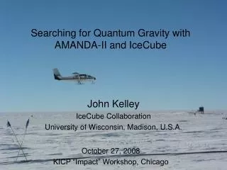
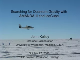
1. Searching for Quantum Gravity with Atmospheric Neutrinos John Kelley December 12, 2008 Thesis Defense

2. Outline • Neutrino detection • New physics signatures • Data selection • Analysis methodology • Results • Outlook

3. Neutrino Detection • Need an interaction — small cross-section necessitates a big target! • Then detect the interaction products (say, by their radiation) charged current  Čerenkov effect

4. Earth’s Transparent Medium: H2O Mediterranean, Lake Baikal Antarctic ice sheet

5. Array of optical modules on cables (“strings” or “lines”) • High energy muon (~TeV) from charged current  interaction • Good angular reconstruction from timing (O(1º)) • Rough  energy estimate from muon energy loss • OR, look for cascades (e, , NC )

6. AMANDA-II • The AMANDA-II neutrino telescope is buried in deep, clear ice, 1500m under the geographic South Pole • 677 optical modules: photomultiplier tubes in glass pressure housings • Muon direction can be reconstructed to within 2-3º optical module

7. Amundsen-Scott South Pole Research Station South Pole Station AMANDA-II skiway Geographic South Pole

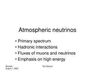
8. Atmospheric Neutrino Production Cosmic rays produce muons, neutrinos through charged pion / kaon decay Even with > km overburden, atm. muon events dominate over  by ~106 Neutrino events: reconstruct direction + use Earth as filter, or look only for UHE events Figure from Los Alamos Science 25 (1997)

9. Current Experimental Status • No detection (yet) of • point sources or other anisotropies • diffuse astrophysical flux • transients (e.g. GRBs, AGN flares, SN) • DM annihilation (Earth or Sun) • Astrophysically interesting limits set • Large sample of atmospheric neutrinos • AMANDA-II: >5K events, 0.1-10 TeV 2000-2006 neutrino skymap, courtesy of J. Braun (publication in preparation) Opportunity for particle physics with high-energy atmospheric 

10. New Physics with Neutrinos? • Neutrinos are already post-Standard Model (massive) • For E > 100 GeV and m < 1 eV, Lorentz > 1011 • Oscillations are a sensitive quantum-mechanical interferometer Eidelman et al.: “It would be surprising if further surprises were not in store…”

11. New Physics Effects • Violation of Lorentz invariance (VLI) in string theory or loop quantum gravity* • Violations of the equivalence principle (different gravitational coupling)† • Interaction of particles with space-time foam  quantum decoherence of flavor states‡ c - 1  c - 2  * see e.g. Carroll et al., PRL 87 14 (2001), Colladay and Kostelecký, PRD 58 116002 (1998) † see e.g. Gasperini, PRD 39 3606 (1989) ‡ see e.g. Anchordoqui et al., hep-ph/0506168

12. “Fried Chicken” VLI • Modified dispersion relation*: • Different maximum attainable velocities ca (MAVs) for different particles: E ~ (c/c)E • For neutrinos: MAV eigenstates not necessarily flavor or mass eigenstates  mixing  VLI oscillations * see Glashow and Coleman, PRD 59 116008 (1999)

13. VLI + Atmospheric Oscillations • For atmospheric , conventional oscillations turn off above ~50 GeV (L/E dependence) • VLI oscillations turn on at high energy (L E dependence), depending on size of c/c, and distort the zenith angle / energy spectrum (other parameters: mixing angle , phase ) González-García, Halzen, and Maltoni, hep-ph/0502223

14. VLI Atmospheric Survival Probability maximal mixing, c/c = 10-27

15. Quantum Decoherence (QD) • Another possible low-energy signature of quantum gravity: quantum decoherence • Heuristic picture: foamy structure of space-time (interactions with virtual black holes) may not preserve certain quantum numbers (like  flavor) • Pure states interact with environment and decohere to mixed states

16. Decoherence + Atmospheric Oscillations characteristic exponential behavior 1:1:1 ratio after decoherence derived from Barenboim, Mavromatos et al. (hep-ph/0603028) Energy dependence depends on phenomenology: n = 3Planck-suppressed operators‡ n = -1 preserves Lorentz invariance n = 2 recoiling D-branes* n = 0 simplest *Ellis et al., hep-th/9704169 ‡ Anchordoqui et al., hep-ph/0506168

17. QD Atmospheric Survival Probability p=1/3

18. Event Selection (2000-2006 data) • Initial data filtering • noise + crosstalk cleaning • bad optical module filtering • fast directional reconstruction, loose “up-going” cut • 80 Hz  0.1 Hz • Final quality cuts • iterative full likelihood reconstruction (timing of photon hits) • cuts on track quality variables • smoothness of hits, angular error estimate, likelihood ratio to downgoing muon fit, space angle between reconstructions, etc. • 0.1 Hz  4 / day (for atm. : 24% eff., 99% purity) • Final sample: 5544 events below horizon (1387 days livetime)

19. Purity Level • Simulating final bit of background not feasible • Estimate contamination by tightening cuts until data/MC ratio stabilizes • Procedure shows essentially no contamination at final cut level (strength = 1) tighter cuts

20. Event 5119326 (May 30, 2005) 199 OMs hit zenith angle 158º angular error 0.7º  energy > ~20 TeV

21. Simulated Observables reconstructed zenith angle Nchannel (energy proxy) QG signature: deficit at high energy, near vertical

22. Testing the Parameter Space Given observables x, want to determine values of parameters {r} that are allowed / excluded at some confidence level Binned likelihood + Feldman-Cousins excluded c/c allowed sin(2)

23. Feldman-Cousins Recipe(frequentist construction) • Test statistic is likelihood ratio: L =LLH at parent {r} - minimum LLH at some {r,best}(compare hypothesis at this point to best-fit hypothesis) • For each point in parameter space {r}, perform many simulated MC “experiments” to see how test statistic varies (close to 2) • For each point {r}, find Lcritat which, say, 90% of the MC experiments have a lower L • Compare Ldatato Lcritat each point to determine exclusion region Feldman & Cousins, PRD 57 7 (1998)

24. Nuisance Parameters / Systematic Errors How to include nuisance parameters {s}: • test statistic becomes profile likelihood • MC experiments use “worst-case” value of nuisance parameters (Feldman’s profile construction method) • specifically, for each r, generate experiments fixing n.p. to data’s , then re-calculate profile likelihood as above

25. Atmospheric Systematics • Separate systematic errors into four classes, depending on effect on observables: • normalization • e.g. atm. flux normalization • slope: change in primary spectrum • e.g. primary CR slope • tilt: tilts zenith angle distribution • e.g. /K ratio • OM sensitivity (large, complicated shape effects) • includes uncertainties in ice properties

26. Systematics Summary error type size method • atm.  flux model norm. ±18% MC study • , - scattering angle norm. ±8% MC study • reconstruction bias norm. -4% MC study • -induced muons norm. +2% MC study • charm contribution norm. +1% MC study • timing residuals norm. ±2% 5-year paper • energy loss norm. ±1% 5-year paper rock density norm. <1% MC study primary CR slope (incl. He) slope  = ±0.03 Gaisser et al. charm (slope) slope  = +0.05 MC study /K ratio tilt tilt +1/-3% MC study charm (tilt) tilt tilt -3% MC study OM sensitivity, ice OM sens. sens. ±10% MC, downgoing 

27. zenith angle number of OMs hit Data consistent with atmospheric neutrinos + O(1%) background Results: Observables

28. Results: VLI upper limit • SuperK+K2K limit*: c/c < 1.9  10-27 (90%CL) • This analysis:c/c < 2.8  10-27 (90%CL) • Limits also set on E2, E3 effects maximal mixing excluded 90%, 95%, 99% allowed CL *González-García & Maltoni, PRD 70 033010 (2004)

29. Results: QD upper limit E2 model (E, E3 limits also set) • SuperK limit‡ (2-flavor): i < 0.9  10-27 GeV-1 (90% CL) • ANTARES sensitivity* (2-flavor): i ~ 10-30GeV-1(3 years, 90% CL) • This analysis:i < 1.3  10-31GeV-1 (90% CL) excluded log10*3,8 / GeV-1 best fit log10*6,7 / GeV-1 * Morgan et al., astro-ph/0412618 ‡ Lisi, Marrone, and Montanino, PRL 85 6 (2000)

30. Conventional Analysis • Parameters of interest: normalization, spectral slope change  relative to Barr et al. • Result: determine atmospheric muon neutrino flux (“forward-folding” approach) best fit best fit 90%, 95%, 99% allowed

31. Translation to Flux Range of allowed flux determined by envelope of curves

32. Result Spectrum this work Blue band: SuperK data, González-García, Maltoni, & Rojo, JHEP 0610 (2006) 075

33. IceCube IceCube South Pole Station AMANDA-II skiway Geographic South Pole

34. 78 74 73 72 67 66 65 59 58 57 56 50 49 48 47 46 40 39 38 30 29 21 Installation Status & Plans AMANDA 2500m deep hole! IceCube string deployed 01/05 IceCube string deployed 12/05 – 01/06 IceCube string and IceTop station deployed 12/06 – 01/07 IceCube string deployed 12/07 – 01/08 IceCube Lab commissioned 40 strings taking physics data Update: 3 of ~16 strings this season

35. Eprimary ~ 1 EeV

36. DOM Calibration • With J. Braun, developed primary DOM calibration software (“DOM-Cal”) • Bootstrap approach calibrates: • front-end amplifier gain • waveform charge vs. time • PMT gain vs. high voltage • PMT transit time vs. high voltage • Entire detector (2500+ DOMs) calibrates itself in parallel in ~1 hour

37. Gain Calibration … … DOMs fit their own single PE charge spectra!

38. IceCube VLI Sensitivity • IceCube: sensitivity of c/c ~ 10-28Up to 700K atmospheric  in 10 years(González-García, Halzen, and Maltoni, hep-ph/0502223) IceCube 10 year

39. Other Possibilities • Extraterrestrial neutrino sources would provide even more powerful probes of QG • GRB neutrino time delay(see, e.g. Amelino-Camelia, gr-qc/0305057) • Electron antineutrino decoherence from, say, Cygnus OB2 (see Anchordoqui et al., hep-ph/0506168) • Hybrid techniques (radio, acoustic) + Deep Core will extend energy reach in both directions

40. Thank you!

41. Violation of Lorentz Invariance (VLI) • Lorentz and/or CPT violation is appealing as a (relatively) low-energy probe of QG • Effective field-theoretic approach by Kostelecký et al. (SME: hep-ph/9809521, hep-ph/0403088) Addition of renormalizable VLI and CPTV+VLI terms; encompasses a number of interesting specific scenarios

42. VLI Phenomenology • Effective Hamiltonian (seesaw + leading order VLI+CPTV): • To narrow possibilities we consider: • rotationally invariant terms (only time component) • only cAB00 ≠ 0 (leads to interesting energy dependence…)

43. Galactic Plane Limits - GeV-1 cm-2 s-1 rad-1 this limit - model (at Earth) GeV-1 cm-2 s-1 sr-1 - Data used: AMANDA 2000-03 Limits include systematic uncertainty of 30% on atm.  flux Energy range: 0.2 to 40 TeV - - - -