Simple Linear Regression
Simple Linear Regression. Often we want to understand the relationships among variables, e.g., SAT scores and college GPA car weight and gas mileage amount of a certain pollutant in wastewater and bacteria growth in local streams

Simple Linear Regression
E N D
Presentation Transcript
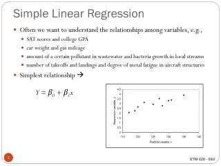
Simple Linear Regression • Often we want to understand the relationships among variables, e.g., • SAT scores and college GPA • car weight and gas mileage • amount of a certain pollutant in wastewater and bacteria growth in local streams • number of takeoffs and landings and degree of metal fatigue in aircraft structures • Simplest relationship Y = β0 + β1x 1 ETM 620 - 09U
Example An electric power cooperative is concerned about the cost of power outages in the winter and the analyst has an idea that these costs are directly related to the average temperature during the outage period. A random sampling of power outages over a number of years was conducted and the cost per 100 homes (adjusted for inflation) was determined, with these results: 2 ETM 620 - 09U
Estimating the regression coefficients • Method of Least Squares • Determine estimates for β0andβ1 so that the sum of the squares of the residuals is minimized, that is … • Solution to the minimization gives: 3 ETM 620 - 09U
For our example, 4 ETM 620 - 09U
What does this mean? • We can draw the regression line that describes the relationship between temperature and outage cost: • We can also predict the cost of outages based on expected temperatures. 5 ETM 620 - 09U
Dangers of regression analysis You can regress any variable on any other variable e.g., hair loss and heart disease; hours playing video games and number of arrests for violent behavior; consecutive hours in class and retention of material; etc. Which of these relationships can you legitimately claim reflect a causal relationship between the “predictor” and the “response”? The regression equation is a “best fit” for the data on which it is based, but may lose validity for predictor values outside the range of the data. For example, our outage cost data implies that the cost per outage decreases as the temperature increases – do you believe that temperatures in the 80’s or 90’s will result in low-cost outages?
How good is our prediction? • Estimating the variance: • Lack of fit test, • Tests the hypotheses H0: the model adequately fits the data H1: the model does not fit the data • As with our goodness-of-fit tests, a high p-value indicates that the model is adequate. 7 ETM 620 - 09U (see next page)
How good is our prediction? • Coefficient of determination, R2 • a measure of the “quality of fit,” or the proportion of the variability explained by the fitted model. • Use with care – increasing the number of variables will usually increase R2, but this doesn’t necessarily make it a “better” model! ETM 620 - 09U 8
Linear regression in Excel … Step 1: Graph the data Does it look like a straight line is the best fit? 9 ETM 620 - 09U
Step 2: Perform the analysis • Choose “Regression” from the Data Analysis menu (under Tools). Input the Y-range (Cost, including the label) and X-range (Temp, including the label), then select • “Labels” if you included those in your data range. • Your desired location for the output. • Residuals and Normal Probability Plot, as desired. • Choose “OK” 10 ETM 620 - 09U
Step 3: Check assumptions • Look at residuals plot and normal probability plots. 11 ETM 620 - 09U
Step 4. Evaluate the results. 12 ETM 620 - 09U
Step 5. Specify and use the model. • Simple linear model: • Use the model to: • Make predictions • expected costs • budgeting • Recommend actions • identify and address sources of cost increase 13 ETM 620 - 09U
In Minitab … • Step 1: Graph the data (for one or two predictor variables)! • Again, do you think a simple linear relationship is the best fit? • Step 2: Select Stat Regression Regression … • Step 3: Choose “Response” (y) and “Predictor” (x). • Step 4: In “Options”, check the “Lack of Fit” box. (“Fit Intercept” box should be checked by default.) Click “OK”. • Step 6: In “Graphs” select the appropriate residual plots to create. • Step 5: Click “OK”. • Step 6: Evaluate the residual plots and results. 14 ETM 620 - 09U
Transformation to a straight line .., If simple linear regression is not appropriate because the underlying function is nonlinear, then we have two choices fit a more complex model transform the model to a straight-line model Simplest transformation – logarithmic transformation Original model: Transformed model:

