Simple Linear Regression

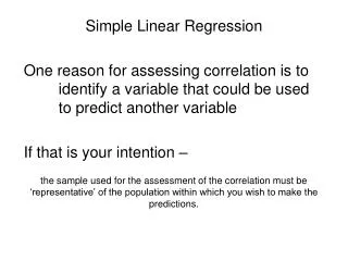
1. Simple Linear Regression Chapter 17

2. 17.1 Introduction • In Chapters 17 to 19 we examine the relationship between interval variables via a mathematical equation. • The motivation for using the technique: • Forecast the value of a dependent variable (y) from the value of independent variables (x1, x2,…xk.). • Analyze the specific relationships between the independent variables and the dependent variable.

3. 17.2 The Model The model has a deterministic and a probabilistic components House Cost Building a house costs about $75 per square foot. House cost = 25000 + 75(Size) Most lots sell for $25,000 House size

4. 17.2 The Model However, house cost vary even among same size houses! Since cost behave unpredictably, we add a random component. House Cost Most lots sell for $25,000 + e House cost = 25000 + 75(Size) House size

5. 17.2 The Model • The first order linear model y = dependent variable x = independent variable b0 = y-intercept b1 = slope of the line e = error variable b0 and b1 are unknown populationparameters, therefore are estimated from the data. y Rise b1 = Rise/Run Run b0 x

6. 17.3 Estimating the Coefficients • The estimates are determined by • drawing a sample from the population of interest, • calculating sample statistics. • producing a straight line that cuts into the data. y w Question: What should be considered a good line? w w w w w w w w w w w w w w x

7. The Least Squares (Regression) Line A good line is one that minimizes the sum of squared differences between the points and the line.

8. Sum of squared differences = (2 -2.5)2 + (4 - 2.5)2 + (1.5 - 2.5)2 + (3.2 - 2.5)2 = 3.99 1 1 The Least Squares (Regression) Line Sum of squared differences = (2 - 1)2 + (4 - 2)2 + (1.5 - 3)2 + (3.2 - 4)2 = 6.89 Let us compare two lines (2,4) 4 The second line is horizontal w (4,3.2) w 3 2.5 2 w (1,2) (3,1.5) w The smaller the sum of squared differences the better the fit of the line to the data. 2 3 4

9. The Estimated Coefficients The regression equation that estimates the equation of the first order linear model is: To calculate the estimates of the line coefficients, that minimize the differences between the data points and the line, use the formulas:

10. Example 17.2 (Xm17-02) The Simple Linear Regression Line • A car dealer wants to find the relationship between the odometer reading and the selling price of used cars. • A random sample of 100 cars is selected, and the data recorded. • Find the regression line. Independent variable x Dependent variable y

11. The Simple Linear Regression Line • Solution • Solving by hand: Calculate a number of statistics where n = 100.

12. The Simple Linear Regression Line • Solution – continued • Using the computer (Xm17-02) Tools > Data Analysis > Regression > [Shade the y range and the x range] > OK

13. The Simple Linear Regression Line Xm17-02

14. Interpreting the Linear Regression -Equation 17067 No data 0 The intercept is b0 = $17067. This is the slope of the line. For each additional mile on the odometer, the price decreases by an average of $0.0623 Do not interpret the intercept as the “Price of cars that have not been driven”

15. 17.4 Error Variable: Required Conditions • The error e is a critical part of the regression model. • Four requirements involving the distribution of e must be satisfied. • The probability distribution of e is normal. • The mean of e is zero: E(e) = 0. • The standard deviation of e is sefor all values of x. • The set of errors associated with different values of y are all independent.

16. E(y|x3) b0 + b1x3 E(y|x2) b0 + b1x2 E(y|x1) b0 + b1x1 The Normality of e The standard deviation remains constant, m3 m2 but the mean value changes with x m1 From the first three assumptions we have: y is normally distributed with mean E(y) = b0 + b1x, and a constant standard deviation se x1 x2 x3

17. 17.5 Assessing the Model • The least squares method will produces a regression line whether or not there are linear relationship between x and y. • Consequently, it is important to assess how well the linear model fits the data. • Several methods are used to assess the model. All are based on the sum of squares for errors, SSE.

18. A shortcut formula Sum of Squares for Errors • This is the sum of differences between the points and the regression line. • It can serve as a measure of how well the line fits the data. SSE is defined by

19. Standard Error of Estimate • The mean error is equal to zero. • If se is small the errors tend to be close to zero (close to the mean error). Then, the model fits the data well. • Therefore, we can, use se as a measure of the suitability of using a linear model. • An estimator of se is given by se

20. It is hard to assess the model based on seeven when compared with the mean value of y. Standard Error of Estimate,Example • Example 17.3 • Calculate the standard error of estimate for Example 17.2, and describe what does it tell you about the model fit? • Solution Calculated before

21. q q q q q q q q q q q q q q q q q q q q q q q q q q q q q q q q q q q q q q q q q q q q q q q q q q q q q q q q q q q q q q q q q q q q q q q q q q q q q q q q q q q q q q q q q q q q q q q q q q q q q q q q q q q q q q Testing the slope • When no linear relationship exists between two variables, the regression line should be horizontal. q q Linear relationship. Linear relationship. Linear relationship. Linear relationship. No linear relationship. Different inputs (x) yield the same output (y). Different inputs (x) yield different outputs (y). The slope is not equal to zero The slope is equal to zero

22. The standard error of b1. Testing the Slope • We can draw inference about b1 from b1 by testing H0: b1 = 0 H1: b1 = 0 (or < 0,or > 0) • The test statistic is • If the error variable is normally distributed, the statistic is Student t distribution with d.f. = n-2. where

23. Testing the Slope,Example • Example 17.4 • Test to determine whether there is enough evidence to infer that there is a linear relationship between the car auction price and the odometer reading for all three-year-old Tauruses, in Example 17.2. Use a = 5%.

24. Testing the Slope,Example • Solving by hand • To compute “t” we need the values of b1 and sb1. • The rejection region is t > t.025 or t < -t.025 with n = n-2 = 98.Approximately, t.025 = 1.984

25. Testing the Slope,Example Xm17-02 • Using the computer There is overwhelming evidence to infer that the odometer reading affects the auction selling price.

26. Coefficient of determination • To measure the strength of the linear relationship we use the coefficient of determination.

27. Explained in part by Remains, in part, unexplained Coefficient of determination • To understand the significance of this coefficient note: The regression model Overall variability in y The error

28. y Coefficient of determination y2 Two data points (x1,y1) and (x2,y2) of a certain sample are shown. Variation in y = SSR + SSE y1 x1 x2 + Unexplained variation (error) Total variation in y = Variation explained by the regression line

29. Coefficient of determination • R2 measures the proportion of the variation in y that is explained by the variation in x. • R2 takes on any value between zero and one. R2 = 1: Perfect match between the line and the data points. R2 = 0: There are no linear relationship between x and y.

30. Coefficient of determination,Example • Example 17.5 • Find the coefficient of determination for Example 17.2; what does this statistic tell you about the model? • Solution • Solving by hand;

31. Coefficient of determination • Using the computerFrom the regression output we have 65% of the variation in the auction selling price is explained by the variation in odometer reading. The rest (35%) remains unexplained by this model.

32. 17.6 Finance Application: Market Model • One of the most important applications of linear regression is the market model. • It is assumed that rate of return on a stock (R) is linearly related to the rate of return on the overall market. R = b0 + b1Rm +e Rate of return on a particular stock Rate of return on some major stock index The beta coefficient measures how sensitive the stock’s rate of return is to changes in the level of the overall market.

33. TheMarket Model, Example Example 17.6 (Xm17-06) • Estimate the market model for Nortel, a stock traded in the Toronto Stock Exchange (TSE). • Data consisted of monthly percentage return for Nortel and monthly percentage return for all the stocks. This is a measure of the stock’s market related risk. In this sample, for each 1% increase in the TSE return, the average increase in Nortel’s return is .8877%. This is a measure of the total market-related risk embedded in the Nortel stock. Specifically, 31.37% of the variation in Nortel’s return are explained by the variation in the TSE’s returns.

34. 17.7 Using the Regression Equation • Before using the regression model, we need to assess how well it fits the data. • If we are satisfied with how well the model fits the data, we can use it to predict the values of y. • To make a prediction we use • Point prediction, and • Interval prediction

35. A point prediction Point Prediction • Example 17.7 • Predict the selling price of a three-year-old Taurus with 40,000 miles on the odometer (Example 17.2). • It is predicted that a 40,000 miles car would sell for $14,575. • How close is this prediction to the real price?

36. The prediction interval • The confidence interval Interval Estimates • Two intervals can be used to discover how closely the predicted value will match the true value of y. • Prediction interval – predicts y for a given value of x, • Confidence interval – estimates the average y for a given x.

37. Interval Estimates,Example • Example 17.7 - continued • Provide an interval estimate for the bidding price on a Ford Taurus with 40,000 miles on the odometer. • Two types of predictions are required: • A prediction for a specific car • An estimate for the average price per car

38. Interval Estimates,Example • Solution • A prediction interval provides the price estimate for a single car: t.025,98 Approximately

39. Interval Estimates,Example • Solution – continued • A confidence interval provides the estimate of the mean price per car for a Ford Taurus with 40,000 miles reading on the odometer. • The confidence interval (95%) =

40. The effect of the given xg on the length of the interval • As xg moves away from x the interval becomes longer. That is, the shortest interval is found at x.

41. The effect of the given xg on the length of the interval • As xg moves away from x the interval becomes longer. That is, the shortest interval is found at x.

42. The effect of the given xg on the length of the interval • As xg moves away from x the interval becomes longer. That is, the shortest interval is found at x.

43. 17.8 Coefficient of Correlation • The coefficient of correlation is used to measure the strength of association between two variables. • The coefficient values range between -1 and 1. • If r = -1 (negative association) or r = +1 (positive association) every point falls on the regression line. • If r = 0 there is no linear pattern. • The coefficient can be used to test for linear relationship between two variables.

44. Y X Testing the coefficient of correlation • To test the coefficient of correlation for linear relationship between X and Y • X and Y must be observational • X and Y are bivariate normally distributed

45. Testing the coefficient of correlation • When no linear relationship exist between the two variables, r = 0. • The hypotheses are: H0: r= 0H1: r¹ 0 • The test statistic is: The statistic is Student t distributed with d.f. = n - 2, provided the variables are bivariate normally distributed.

46. Testing the Coefficient of correlation • Foreign Index Funds (Index) • A certain investor prefers the investment in an index mutual funds constructed by buying a wide assortment of stocks. • The investor decides to avoid the investment in a Japanese index fund if it is strongly correlated with an American index fund that he owns. • From the data shown in Index.xls should he avoid the investment in the Japanese index fund?

47. Testing the Coefficient of correlation • Foreign Index Funds • A certain investor prefers the investment in an index mutual funds constructed by buying a wide assortment of stocks. • The investor decides to avoid the investment in a Japanese index fund if it is strongly correlated with an American index fund that he owns. • From the data shown in Index.xls should he avoid the investment in the Japanese index fund?

48. Testing the Coefficient of Correlation,Example • Solution • Problem objective: Analyze relationship between two interval variables. • The two variables are observational (the return for each fund was not controlled). • We are interested in whether there is a linear relationship between the two variables, thus, we need to test the coefficient of correlation

49. The value of the t statistic is Conclusion: There is sufficient evidence at a = 5% to infer that there are linear relationship between the two variables. Testing the Coefficient of Correlation,Example • Solution – continued • The hypothesesH0: r= 0H1: r¹ 0. • Solving by hand: • The rejection region:|t| > ta/2,n-2 = t.025,59-2» 2.000. • The sample coefficient of correlation: Cov(x,y) = .001279; sx = .0509; sy = 0512 r = cov(x,y)/sxsy=.491

50. Testing the Coefficient of Correlation,Example • Excel solution (Index)