Octopus Arm Project
Octopus Arm Project. Final Presentation. Dmitry Volkinshtein & Peter Szabo. Supervised by: Yaki Engel. Contents. Project Goal The Octopus and its Arm Octopus Arm Model Reinforcement Learning On-Line GPTD Algorithm System Implementation Debug and Testing

Octopus Arm Project
E N D
Presentation Transcript
Octopus Arm Project Final Presentation Dmitry Volkinshtein & Peter Szabo Supervised by: Yaki Engel
Contents • Project Goal • The Octopus and its Arm • Octopus Arm Model • Reinforcement Learning • On-Line GPTD Algorithm • System Implementation • Debug and Testing • Learning Process • Challenges and Problems • Results • Conclusions
1. Project Goal Teach a 2D octopus arm model to reach a given point in space by novel means of reinforcement learning.
2. The Octopus and its Arm(1/2) An Octopus is a carnivorous eight-armed sea creature with a large soft head and two rows of suckers on the underside of each arm (usually lives on the bottom of the ocean).
2. The Octopus and its Arm(2/2) An Octopus Arm is a muscular hydrostat organ capable of exerting force with the sole use of muscles, without requiring a rigid skeleton.
3. Octopus Arm Model(1/3) The octopus arm’s model is the outcome of a previous project in this lab. It is a 2D model written in C. We have upgraded it to C++ and added some features for better performance and compliance with other parts of our project.
3. Octopus Arm Model(2/3) The model simulates the physical behavior of the arm in its natural environment, considering: • Muscle forces. • Internal forces (keeping the constant volume of the arm, which is filled with fluids). • Gravitation and the floatation vertical forces. • Drag forces caused by the water.
3. Octopus Arm Model(3/3) The model approximates the continuous octopus arm by dividing it into segments and calculating the forces on each segment separately.
4. Reinforcement Learning (1/4) Reinforcement Learning(RL) Learning a behavior through trial and error interactions with a dynamic environment. Basic RL Definitions Agent - A learning and decision making entity. Environment - An entity the agent interacts with, comprising everything that cannot be changed arbitrarily by the agent.
4. Reinforcement Learning (2/4) Basic RL Definitions (cont.) State - The condition of the environment. Action - A choice made by the agent, based on the state. Reward - The input upon which the actions are evaluated by the agent.
4. Reinforcement Learning (3/4) The agent uses two functions to produce its next action: Value - For a given state X, the Value function is the expectation sum of rewards when the agent starts from X and uses the current Policy. Policy - For a given Value function, the Policy function returns the action to take when the agent is located in state X.
4. Reinforcement Learning (4/4) In our case: • The State is the location and speed of all the vertexes in the arm. An arm represented by N segments will have 2(N+1) vertexes and 8(N+1) dimensions. • The Action is a muscle activation in the arm, chosen by the agent module from a finite and constant set of activations. • The Environment is the arm simulation that provides the result of the activation (the next state of the arm). • The Reward the agent gets is state dependant, and set according to the proximity between arm and goal. • The Agent is an On-Line GPTD based learning module.
5. On-Line GPTD Algorithm(1/3) TD(l) - An algorithm family in which temporal differences are used to estimate the value function on-line. GPTD - Gaussian Processes for TD Learning: Assuming the sequence of rewards is a Gaussian random process (with noise), and the rewards are samples of that process, we can estimate the value function using Gaussian estimation and a kernel function.
5. On-Line GPTD Algorithm(2/3) GPTD disadvantages: • Space consumption of O(t2). • Time consumption of O(t3). The proposed solution: On-Line Sparsification applied on the GPTD algorithm. Instead of keeping a large number of results of a vector function, we keep a dictionary of input vectors that can span, up to an accuracy threshold, the original vector function’s space.
5. On-Line GPTD Algorithm(3/3) Applying on-line sparsification on GPTD yields: • Recursive update rules. • No matrix inversion needed. • Matrix dimensions depend on mt (dictionary size at time t), which is generally not linear in t. Using this, we can calculate: • Value estimate with O(mt) time. • Value variance with O(mt2) time. • Each dictionary update with O(mt2) time.
6. System Implementation(1/5) Environment 3 Octopus Arm Simulation Rewarder 4 4 3 Agent 3 Explorer (OPI / Actor-Critic) On-Line GPTD 5 2 1
6. System Implementation(2/5) The Agent • Uses the On-line GPTD algorithm for value estimation. • Policy by one of the following: • Optimistic Policy Iteration (OPI). In this case there is a choice between two methods: • The e- greedy policy: • The Softmax policy: • Actor-Critic - By using two GPTD instances. • Interval Estimation - Greedy over:
6. System Implementation(3/5) The GPTD algorithm’s two versions • Deterministic - Calculates value for an MDP with deterministic state transitions. • Works better with Actor-Critic. • Relatively fast convergence. • Stochastic - Calculates value for an MDP with stochastic state transitions. • Works better with Softmax and e - greedy. • Slow convergence (more parameters).
6. System Implementation(4/5) Goal types • The goal is a small circular zone in the 2D space. • It can be reached in two predefined ways: • With the tip of the arm. • With any vertex along the arm. • In both cases it can be reached with either side of the arm (dorsal or ventral). • A speed limit can be applied, i.e. reaching the goal zone faster than limit will not count as goal.
6. System Implementation(5/5) The Rewarder There are three types of rewarding: • Discrete: • Exponential: • Negative exponential: In all cases: • Hitting an obstacle yields a reward of , and ends the trial. • A penalty proportional to the arm’s energy consumption in the last transition is reduced from the reward.
7. Debug and Testing • GPTD implementation included the non-recursive version of the algorithm (used only for debugging). • We tested GPTD (both deterministic and stochastic) on a discrete maze and witnessed correct value convergence. • We tested the system with a short, degenerate arm of 3 segments. • We ran the system in Supervised Learning mode (with g=0) and witnessed the value converging to the reward function.
8. Learning Process(1/4) Agent’s Learning • Running a large number (~103-104) of consecutive learning trials. Each trial starts from a random initial state. • Saving GPTD parameters each N-th trial.
8. Learning Process(2/4) Agent’s Performance Measurement • Creating a pool of evenly distributed arm states. • Loading each N-th GPTD save. • Running greedy policy over the manifold of initial states, noting whether and when was the goal reached. • Merging the raw data to statistics - goal percentage for each GPTD save, and goal times for each initial state.
8. Learning Process(3/4) Parameters’ Calibration Simulation • Time - Total time, interval between activations. • Activations - Total number and types. GPTD • Stochastic vs. Deterministic • General parameters - s02, n, g, l • Kernel function - Gaussian, Polynomial
8. Learning Process(4/4) Parameters’ Calibration (cont.) Exploration • OPI - Softmax temperature, e - greedy descent factors. • Actor-Critic - Trial interval between GPTD switches. • Interval Estimation - Variance multiplying factor. Reward Function • Discrete vs. Exponential • Energy penalty factor • Obstacles Goal • Size • Location • Speed limit
9. Challenges and Problems • A 10 segment arm has 88 dimensions. It uses a huge amount of memory and lengthens simulation time. Solution: Occupy all of the lab’s available computers for months. • Too many activations cause greedy moves to consume a lot of time. Solution: Creating a small set of activations, yet one that still supports the arm’s full range of movement. • GPTD is an estimator for an MDP value function. If we use OPI, the policy is not MDP. Solution: Forgetfulness (l) or Actor-Critic. • Starting from a random state improves learning, yet a random state’s production on-line is problematic with our simulation. Solution: Selecting random states from GPTD’s dictionary, and using the less visited amongst them.
10. Results (1/8) 10 Segment Arm - OPI, Gaussian Kernel
10. Results (2/8) 10 Segment Arm - OPI, Polynomial Kernel
10. Results (3/8) 10 Segment Arm - OPI, Polynomial Kernel
10. Results (4/8) 10 Segment Arm - OPI, Polynomial Kernel 92%
10. Results (5/8) 10 Segment Arm - OPI, Polynomial Kernel 96%
10. Results (6/8) 10 Segment Arm - OPI, Polynomial Kernel 90%
10. Results (7/8) 10 Segment Arm - Actor-Critic, Gaussian Kernel 96%
10. Results (8/8) Summary • OPI yields a peak performance of 96%. • Actor-Critic yields a peak performance of 96%. GOAL !!! GOAL !!! GOAL !!!
11. Conclusions(1/2) • It is evident that the arm has gone through a significant learning process. Though not to perfection, but the arm clearly improved its behavior, from random movements to goal oriented movements. • OPI and Actor-Critic both prove to be effective learning strategies. Some further investigation is needed to establish the performance differences between the two. • Despite some disappointing results, we are optimistic (hence still using OPI ;-). We believe that further fine-tuning of system parameters, and providing longer training time will result in a more decisive convergence.
11. Conclusions(2/2) • The system’s large number of dimensions slows down the simulation and inflates the dictionary. This is the current bottleneck of the learning process. More computing power is needed for a reasonable learning time. • Based on our latest results, we believe we will establish that On-Line GPTD is practical algorithm which tackles successfully, and with moderate computing resources, the difficult problem of reinforcement learning in a continuous state space with vast number of dimensions.