Download
1 / 73
730 likes | 748 Vues
This article discusses the modeling of volatility skews in equity markets, with a focus on the negative skew observed since the 1987 crash. It explores the reasons for volatility skews and presents different modeling approaches, including local volatility models and stochastic volatility models. Theoretical methods for calculating break-even volatilities and understanding the relationship between spot prices and volatility are also discussed.

E N D
Modelling Volatility Skews Bruno Dupire Bloomberg bdupire@bloomberg.net London, November 17, 2006
OUTLINE Generalities Leverage and jumps Break-even volatilities Volatility models Forward Skew Smile arbitrage
K K K Market Skews Dominating fact since 1987 crash: strong negative skew on Equity Markets Not a general phenomenon Gold: FX: We focus on Equity Markets
Skews • Volatility Skew: slope of implied volatility as a function of Strike • Link with Skewness (asymmetry) of the Risk Neutral density function ?
Market Skew Supply and Demand Th. Skew K Why Volatility Skews? • Market prices governed by • a) Anticipated dynamics (future behavior of volatility or jumps) • b) Supply and Demand • To “ arbitrage” European options, estimate a) to capture risk premium b) • To “arbitrage” (or correctly price) exotics, find Risk Neutral dynamics calibrated to the market
S t t S Modeling Uncertainty Main ingredients for spot modeling • Many small shocks: Brownian Motion (continuous prices) • A few big shocks: Poisson process (jumps)
K 2 mechanisms to produce Skews (1) • To obtain downward sloping implied volatilities • a) Negative link between prices and volatility • Deterministic dependency (Local Volatility Model) • Or negative correlation (Stochastic volatility Model) • b) Downward jumps
2 mechanisms to produce Skews (2) • a) Negative link between prices and volatility • b) Downward jumps
t0 t1 t2 x = St1-St0 y = St2-St1 Option prices Option prices FWD variance Δ Hedge Δ Hedge Leverage FWD skewness Dissociating Jump & Leverage effects • Variance : • Skewness :
Dissociating Jump & Leverage effects • Define a time window to calculate effects from jumps and • Leverage. For example, take close prices for 3 months • Jump: • Leverage:
Theoretical Skew from Prices ? => • Problem : How to compute option prices on an underlying without options? • For instance : compute 3 month 5% OTM Call from price history only. • Discounted average of the historical Intrinsic Values. • Bad : depends on bull/bear, no call/put parity. • Generate paths by sampling 1 day return recentered histogram. • Problem : CLT => converges quickly to same volatility for all strike/maturity; breaks autocorrelation and vol/spot dependency.
Theoretical Skew from Prices (2) • Discounted average of the Intrinsic Value from recentered 3 month histogram. • Δ-Hedging : compute the implied volatility which makes the Δ-hedging a fair game.
S K t Theoretical Skewfrom historical prices (3) How to get a theoretical Skew just from spot price history? Example: 3 month daily data 1 strike • a) price and delta hedge for a given within Black-Scholes model • b) compute the associated final Profit & Loss: • c) solve for • d) repeat a) b) c) for general time period and average • e) repeat a) b) c) and d) to get the “theoretical Skew”
Strike dependency • BE volatility is an average of returns, weighted by the Gammas, which depend on the strike
One Single Model • We know that a model with dS = s(S,t)dW would generate smiles. • Can we find s(S,t) which fits market smiles? • Are there several solutions? ANSWER: One and only one way to do it.
Risk NeutralProcesses Diffusions Compatible with Smile The Risk-Neutral Solution But if drift imposed (by risk-neutrality), uniqueness of the solution
Forward Equation • BWD Equation: price of one option for different • FWD Equation: price of all options for current • Advantage of FWD equation: • If local volatilities known, fast computation of implied volatility surface, • If current implied volatility surface known, extraction of local volatilities:
Forward Equations (2) • Several ways to obtain them: • Fokker-Planck equation: • Integrate twice Kolmogorov Forward Equation • Tanaka formula: • Expectation of local time • Replication • Replication portfolio gives a much more financial insight
Volatility Expansion • K,T fixed. C0 price with LVM • Real dynamics: • Ito • Taking expectation: • Equality for all (K,T)
Summary of LVM Properties is the initial volatility surface • compatible with local vol • compatible with (calibrated SVM are noisy versions of LVM) • deterministic function of (S,t) (if no jumps) future smile = FWD smile from local vol • Extracts the notion of FWD vol (Conditional Instantaneous Forward Variance)
Heston Model Solved by Fourier transform:
Role of parameters • Correlation gives the short term skew • Mean reversion level determines the long term value of volatility • Mean reversion strength • Determine the term structure of volatility • Dampens the skew for longer maturities • Volvol gives convexity to implied vol • Functional dependency on S has a similar effect to correlation
s s ST ST Spot dependency • 2 ways to generate skew in a stochastic vol model • Mostly equivalent: similar (St,st) patterns, similar future • evolutions • 1) more flexible (and arbitrary!) than 2) • For short horizons: stoch vol model local vol model + independent noise on vol.
SABR model • F: Forward price with correlation r
SABR fallacy • SABR claims to dissociate vol dynamics from Skew fitting • Many banks manage their vol risk with SABR • BUT if 2 SABR models fit the same skew, they generate essentially the same vol dynamics, which coincide in average with LVM dynamics!
Calibration according to SABR Backbone: as a function of F with frozen depends only on Many banks calibrate by: 1) Estimating from historical backbone 2) Then adjusting to fit the skew
Problems • Freezing ignores which actually impacts the average backbone • SABR can be rewritten with the lognormal volatility • In this parameterization instead of , freezing gives : the backbone is then constant! The backbone depends on the parameterization , it is not intrinsic to the model: it is a flawed concept