by Nannapaneni Narayana Rao Edward C. Jordan Professor Emeritus of Electrical and Computer Engineering University of Ill

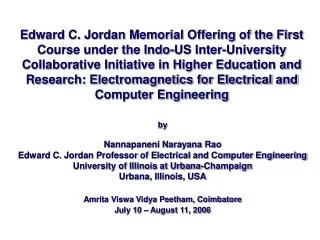
1. Fundamentals of Electromagnetics:A Two-Week, 8-Day, Intensive Course for Training Faculty in Electrical-, Electronics-, Communication-, and Computer- Related Engineering Departments by Nannapaneni Narayana Rao Edward C. Jordan Professor Emeritus of Electrical and Computer Engineering University of Illinois at Urbana-Champaign, USA Distinguished Amrita Professor of Engineering Amrita Vishwa Vidyapeetham, India Amrita Viswa Vidya Peetham, Coimbatore August 11, 12, 13, 14, 18, 19, 20, and 21, 2008

2. × ò ò D d S = r dv S V Maxwell’s Equations d × × ò E d l = – ò B d S dt C S Charge density Magnetic flux density Electric field intensity d × × × × ò B d S = 0 ò ò ò H d l = J d S + D d S dt S C S S Current density Magnetic field intensity Displacement flux density

3. Module 1 Vectors and Fields Vector algebra Caresian coordinate system Cylindrical and spherical coordinate systems Scalar and vector fields Sinusoidally time-varying fields The electric field The magnetic field Lorentz force equation

4. Instructional Objectives Identify the polarization of a sinusoidally time-varying vector field Calculate the electric field due to a charge distribution by applying superposition in conjunction with the electric field due to a point charge Calculate the magnetic field due to a current distribution by applying superposition in conjunction with the magnetic field due to a current element Apply Lorentz force equation to find the electric and magnetic fields, for a specified set of forces on a charged particle moving in the field region

5. Vector Algebra (FEME, Sec. 1.1; EEE6E, Sec. 1.1) In this series of PowerPoint presentations, FEME refers to “Fundamentals of Electromagnetics for Electrical and Computer Engineering,” U.S. and International Editions (2009), or “Fundamentals of Electromagnetics for Engineering,” Indian Edition (2009), and EEE6E refers to “Elements of Engineering Electromagnetics, 6th Edition,” U.S. and International Editions (2004) or Indian Edition (2006).

6. (1)Vectors (A) vs. Scalars (A) Magnitude and direction Magnitude only Ex: Velocity, Force Ex: Mass, Charge (2)Unit Vectors have magnitude unity denoted by symbol a with subscript Useful for expressing vectors in terms of their components.

7. (3)Dot Product is a scalar A A • B = AB cos a B Useful for finding angle between two vectors.

8. (4)Cross Product is a vector A A B = AB sin a B is perpendicular to both A and B. Useful for finding unit vector perpendicular to two vectors. an

9. where (5)Triple Cross Product in general.

10. (6)Scalar Triple Product is a scalar.

11. Volume of the parallelepiped

12. D1.2 (EEE)A = 3a1 + 2a2 + a3 B = a1 + a2 – a3 C = a1 + 2a2 + 3a3 (a)A + B – 4C = (3 + 1 – 4)a1 + (2 +1 – 8)a2 + (1 – 1 – 12)a3 = – 5a2 – 12a3

13. (b)A + 2B – C = (3 + 2 – 1)a1 + (2 + 2 – 2)a2 + (1 – 2 + 3)a3 = 4a1 + 2a2 – 4a3 Unit Vector = =

14. (c)A • C = 3 1 + 2 2 + 1 3 = 10 (d) = = 5a1 – 4a2 + a3

15. (e) = 15 – 8 + 1 = 8 Same as A • (B C) = (3a1 + 2a2 + a3) • (5a1 – 4a2 + a3) = 3 5 + 2 (–4) + 1 1 = 15 – 8 + 1 = 8

16. P1.5 (EEE) D = B – A ( A + D = B) E = C – B ( B + E = C) D and E lie along a straight line.

17. What is the geometric interpretation of this result?

18. Another Example Given Find A.

19. To find C, use (1) or (2).

20. Cartesian Coordinate System (FEME, Sec. 1.2; EEE6E, Sec. 1.2)

21. Cartesian Coordinate System

22. Right-handed system xyz xy… ax, ay, az are uniform unit vectors, that is, the direction of each unit vector is same everywhere in space.

23. (1)

25. P1.8A(12, 0, 0), B(0, 15, 0), C(0, 0, –20). (a) Distance from B to C = = (b) Component of vector from A to C along vector from B to C = Vector from A to C • Unit vector along vector from B to C

26. (c) Perpendicular distance from A to the line through B and C =

27. = = (2)Differential Length Vector (dl)

28. dl = dx ax + dy ay = dx ax + f¢(x) dx ay Unit vector normal to a surface:

29. D1.5 Find dl along the line and having the projection dz on the z-axis. (a) (b)

30. (c) Line passing through (0, 2, 0) and (0, 0, 1).

31. (3)Differential Surface Vector (dS) Orientation of the surface is defined uniquely by the normal ± an to the surface. For example, in Cartesian coordinates, dS in any plane parallel to the xy plane is

32. (4)Differential Volume (dv) In Cartesian coordinates,

33. Cylindrical and Spherical Coordinate Systems (FEME, Appendix A; EEE6E, Sec. 1.3)

34. Cylindrical Coordinate System

35. Spherical Coordinate System

36. 1-35 Cylindrical and Spherical Coordinate Systems Cylindrical (r, f, z) Spherical (r, q, f) Only az is uniform. All three unit ar and af are vectors are nonuniform. nonuniform.

37. x = r cos fx = r sin q cos f y = r sin fy = r sin q sin f z = zz = r cos q D1.7 (a) (2, 5p/6, 3) in cylindrical coordinates

38. (b)

39. (c)

40. (d)

41. Conversion of vectors between coordinate systems

42. P1.18A = ar at (2, p/6, p/ 2) B = aq at (1, p/3, 0) C = af at (3, p/4, 3p/2)

44. (a) (b) 1-43

45. (c) (d)

46. Differential Length Vectors: Cylindrical Coordinates: dl = drar + rdfaf +dz az Spherical Coordinates: dl = drar + rdqaq + r sin qdfaf

47. Scalar and Vector Fields (FEME, Sec. 1.3; EEE6E, Sec. 1.4)

48. FIELD is a description of how a physical quantity varies from one point to another in the region of the field (and with time). (a)Scalar fields Ex: Depth of a lake, d(x, y) Temperature in a room, T(x, y, z) Depicted graphically by constant magnitude contours or surfaces.

49. (b)Vector Fields Ex: Velocity of points on a rotating disk v(x, y) = vx(x, y)ax + vy(x, y)ay Force field in three dimensions F(x, y, z) = Fx(x, y, z)ax + Fy(x, y, z)ay + Fz(x, y, z)az Depicted graphically by constant magnitude contours or surfaces, and direction lines (or stream lines).

50. Example: Linear velocity vector field of points on a rotating disk