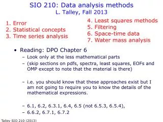
SIO 210: Data analysis methods L. Talley, Fall 2013
SIO 210: Data analysis methods L. Talley, Fall 2013. Reading: DPO Chapter 6 Look only at the less mathematical parts (skip sections on pdfs, spectra, least squares, EOFs and OMP except to note that the material is there)

SIO 210: Data analysis methods L. Talley, Fall 2013
E N D
Presentation Transcript
SIO 210: Data analysis methodsL. Talley, Fall 2013 • Reading: DPO Chapter 6 • Look only at the less mathematical parts • (skip sections on pdfs, spectra, least squares, EOFs and OMP except to note that the material is there) • i.e. you should know that these approaches exist but I am not going to require you to know the details of the mathematical expressions. • 6.1, 6.2, 6.3.1, 6.4, 6.5 (not 6.5.3, 6.5.4), • 6.6.2, 6.7.1, 6.7.2 4. Least squares methods 5. Filtering 6. Space-time data 7. Water mass analysis 1. Error 2. Statistical concepts 3. Time series analysis Talley SIO 210 (2013)
1. (Sampling and error review) • Sampling • Synoptic sampling • Time series • Discrete measurements, finite record length • Error: • Accuracy: error relative to absolute standard • Precision: error within data set, or associated with instrument noise/resolution Talley SIO 210 (2013)
1. Random and systematic error Random error: fluctuations (in either direction) of measured values due to precision limitations of the measurement device. Random error is quantified by the variance or standard deviation. (PRECISION) Systematic error (bias): offset, high or low, which cannot be determined through statistical methods used on the measurements themselves. An oceanographic example: Two or more technical groups measure the same parameters (e.g. temperature, nutrients or oxygen, etc). The mean values the groups obtain differ because of differences in methods, chemical standards, etc. Error can only be evaluated by comparison of the two sets of measurements with each other or with an absolute standard. (ACCURACY) Talley SIO 210 (2013)
2. Basic concepts: Mean, variance, standard deviation, standard error • Mean: • Anomaly: x = xmean + xanomaly ; therefore xanomaly = x-xmean • Variance: • Standard deviation of the measurements: • Standard error: /√N Talley SIO 210 (2013)
2. Standard deviation vs. standard error Standard deviation is a measure of variability in the field that is measured. Standard error is a measure of how well the field is sampled. Salinity at 500 m Sampling Standard deviation Standard error Talley SIO 210 (2013)
2. Climatologies Climatology (mean): mean field based on large data base, usually covering many years Climatology (Reynolds October Mean Observed Field (Oct. 2012) Anomaly: Oct. 2012 Minus Reynolds October climatology http://www.pmel.noaa.gov/tao/ Talley SIO 210 (2013)
3. Time series analysis A time series is a data set collected as a function of time Examples: current meter records, sea level records, temperature at the end of the SIO pier Some common analysis methods: Display the data (simple plot)! (always useful) Mean, variance, standard deviation, etc. Correlation of different time series with each other Spectral (Fourier) analysis of a time series to determine its frequency distributions. Underlying concept is that any time series can be decomposed into a continuous set of sinusoidal functions of varying frequency. Spectrum: amplitude of each of the frequency components. Very useful for detecting things like tides, inertial motions, that have specific forcing frequencies. Talley SIO 210 (2013)
3A. Display time series data: aHovmöller diagram (time on one axis, space on the other) Equatorial Pacific sea level height anomaly from satellite (High sea level anomaly - El Nino!) (Low propagating west to east) Talley SIO 210 (2013)
3.C. Time series analysis Correlation: integral of the product of two time series, can be with a time lag. (Autocorrelation is the time series with itself with a time lag.) • Integral time scale: time scale of the autocorrelation (definitions vary) – crude definition might be at what time lag does the autocorrelation drop to zero (which is the decorrelation timescale) (First calculate the autocorrelation for a large number of time lags.) • Degrees of freedom: total length of record divided by the integral time scale – that gives how many realizations of the phenomenon you have. Good to have about 10. Talley SIO 210 (2013)
3.C. Covariance and correlation Covariance: how two variables are related statistically. Correlation: covariance divided by the product of the (sample) standard deviations of the two variables. Correlations have values from 0 to 1. How to tell if a correlation is significant? Talley SIO 210 (2013)
3.C. Time series analysis: example Example of correlation of different time series with each other North Atlantic Oscillation index (time series) Correlation with surface temperature and with surface pressure (done at each point, so each lat/lon gives a time series to correlate with NAO index) Talley SIO 210 (2013)
3.C. Autocorrelation and timescales (a) Time series of temperature at Fanning Island (Pacific Ocean) from the NCAR Community Ocean Model. (b) Autocorrelation normalized to a maximum value of 1 (biased estimate with averages divided by N). (c and d) Autocorrelation (unbiased estimate with averages divided by N–n). Source: From Gille (2005). Decorrelation time scale: 1st 0 crossing. Integral time scale is a little longer (based on integral of the autocorrelation) DPO FIGURE 6.2 Talley SIO 210 (2013)
3.D. Time series analysis Spectra: Limitations are imposed by sampling interval. The highest frequency that can be resolved in the spectrum(called the “Nyquist frequency”) is 1/2t where t is the sampling interval. Any energy at higher frequencies becomes “aliased” into lower frequencies, causing error in their amplitude estimates. length of the total record. Generally should have about 10 realizations of a given frequency for the amplitude to be significant. Can prove difficult when trying to detect climate change for instance. This is related to “degrees of freedom”. Talley SIO 210 (2013)
3.D. Fundamental frequency and Nyquist frequency: sources of error in time series analysis Sampling: N samples at time interval Δt. Length of time series is then T = NΔt • Fundamental frequency • The lowest frequency that is resolved is • f = 1/T = 1/NΔt • Nyquist frequency • The highest frequency that is resolved is • f = 1/2Δt Talley SIO 210 (2013)
3.D. Nyquist frequency and aliasing Aliasing: what happens to high frequencies that are above the Nyquist frequency cutoff? They are in the record, and are sampled, but not resolvable because their frequency content is not resolved They are aliased to a lower frequency. Talley SIO 210 (2013)
4. Least squares methods These are methods for mapping (time-dependent and spatially-dependent) data, filling in gaps, bringing prior information to bear on how one maps • Objective mapping • Data assimilation (merging data and computer models) (no info given here) • Inverse methods (finding “optimal” solution given sparse or incomplete data) (no info given here) Talley SIO 210 (2013)
4.A. Spatial sampling: Objective analysis Many oceanographic data are collected in several spatial dimensions. Sample separations are very irregular. We want to interpolate these in an optimal way to a grid for plotting and comparison with other data sets. Objective analysis is a method for interpolating. It requires prior knowledge of the spatial correlation scales of the data to be mapped; since these would normally be calculated from the data themselves, they are often chosen in an ad hoc fashion. Talley SIO 210 (2013)
4.A. Oceanographic sampling: objective mapping in the vertical Discrete bottle samples: objectively mapped to uniform grid in vertical (10 m) and horizontal (10 km) WOCE Pacific atlas (Talley, 2007) Talley SIO 210 (2013)
4.A. Oceanographic sampling: Vertical sections • Vertical coordinates: • Depth (pressure) • Potential density or neutral density (or theta) Talley SIO 210 (2013)
4.A. Oceanographic sampling: Mapping in the horizontal • Original station data: objectively mapped to a regular grid (NOAA/NODC) • Different types of surfaces that are commonly used: • Constant depth • Isopycnal • “core layer” – here salinity maximum DPO Fig. 6.4 Talley SIO 210 (2013)
5. Filtering Time series or spatial sampling includes phenomena at frequencies that may not be of interest (examples: want inertial mode but sampling includes seasonal, surface waves, etc.) Use various filtering methods (running means with “windows” or more complicated methods of reconstructing time series) to isolate frequency of interest Example: Time series of a climate index with 1-year and 5-year running means as filters. Talley SIO 210 (2013)
6. Space-time sampling: empirical orthogonal functions etc Underlying physical processes might not be best characterized by sines and cosines, especially in the spatial domain. They may be better characterized by functions that look like the basin or circulation geometries. Empirical orthogonal function analysis: let the data decide what the basic (orthogonal) functions are that add to give the observed values. Basic EOF analysis: obtain spatial EOFs with a time series of amplitude for each EOF. (The time series itself could be Fourier-analyzed if desired.) Talley SIO 210 (2013)
6. EOF example: Southern Annular Mode Modes of decadal (climate) variability NAM Talley SIO 210 (2013)
7. Water mass analysis • Property-property relations (e.g., theta-S) • Volumetric property-property • Optimum multiparameter analysis (OMP) Talley SIO 210 (2013)
7. Potential temperature-salinity at 25°W Talley SIO 210 (2013)
7. Water mass analysis: volumetric potential temperature-salinity Talley SIO 210 (2013)
7. Optimum multiparameter analysis (OMP) Use of water properties (T, S, oxygen, nutrients, other tracers): define source waters in terms of properties, then use a least squares analysis to assign every observation to a proportion of each source water Example of NADW vs. AABW: fractions of each (Johnson et al., 2008) DPO 14.15 Talley SIO 210 (2013)