WEEK-2 THE EARTH SYSTEM: LITHOSPHERE-HYDROPHERE INTERACTIONS
480 likes | 501 Vues
This article provides an overview of the Earth's layers and their classification based on physical properties and composition. It explores the different types of rocks in the Earth's crust and their formation processes. The article also discusses the distribution of chemical elements in rocks and how we can predict their occurrence.

WEEK-2 THE EARTH SYSTEM: LITHOSPHERE-HYDROPHERE INTERACTIONS
E N D
Presentation Transcript
Environmental Biogeochemistry of Trace metals (CWR6252) WEEK-2THE EARTH SYSTEM: LITHOSPHERE-HYDROPHERE INTERACTIONS
I - Earth’s LayersClassification based on physical properties and composition • CRUST • Solid Rocks • MANTLE • Molten Rocks • OUTER CORE • Liquid-like • Ni and Fe • INNER CORE • Solid • dominated by Ni and Fe • Seismic compressional waves (P)all media • 2. Seismic shear waves (S)solid only
The Earth's Crustis like the skin of an apple. It is very thin in comparison to the other three layers. • About 3-5 miles (8 kilometers) thick under the oceans (oceanic crust) and about 25 miles (32 kilometers) thick under the continents (continental crust). • The temperatures of the crust vary from air temperature on top to about 1600 degrees Fahrenheit (or 8700C) in the deepest parts of the crust. • It is made of solid rocks
WHAT ARE ROCKS? • Rocks are cohesive aggregates made up of one or more minerals. • Minerals are homogeneous, naturally occurring, inorganic solids with well-defined chemical composition and a characteristic crystalline structure. A mineral may be a single element or a compound made up of a number of elements.
1. Igneous Rocks Extrusive igneous rocks: • Natural Glass—very fast lava cooling at the Earth’s surface – No mineral crystal formed • Volcanic rocks—fast cooling of the lava at or near surface to produce dark rocks. BASALT is the most common extrusive IR found in sea floor and locations of cooling magma on continents [Minerals: olivines, Pyroxenes, amphiboles, Plagioclase feldspar, Alkali feldspar, and quartz. [Fe, Mg, Ca, Si, Na, K, Al, O, H] Intrusive or PLUTONIC ROCKS: formed by slow cooling of the magma deep in the crust resulting in the formation of light pink igneous rocks (e.g. granite, gabbro, granodiorite). The slow cooling process allows the formation of big mineral crystals. Minerals: olivines, Pyroxenes, amphiboles, Plagioclase feldspar, Alkali feldspar, and quartz. [Fe, Mg, Ca, Si, Na, K, Al, O, H] MANTLE: RISING MAGMA
2. Sedimentary Rocks Formed at low temperature by LITHIFICATION, a set of processes transforming sediments to sedimentary rocks. sedimentary rock types include: 2.1. Clastic Sedimentary Rocks [from Greek “klastos” = broken] are made from the broken bits of other rocks. 2.3. Organic Sedimentary Rocks: cemented remains of living things such as clamshells, plankton skeletons, dinosaur bones, and plants. 2.2. Chemical Sedimentary Rocks: formed only by precipitation or growth from solutions
3. Metamorphic Rocks Metamorphic rocks are formed where plates are coming together; rocks are heated and are under high pressure. D C Contact Metamorphism Regional Metamorphism
GRANITE Schist
II - DISTRIBUTION OF CHEMICAL ELEMNTS IN ROCKS HOW CAN WE PREDICT THE OCCURRENCE / DISTRIBUTION OF CHEMICAL ELEMENTS IN GEOLOGICAL MATERIALS? EXAMPLE 1: THE PERIODIC TABLE AS A PREDICTIVE TOOL EXAMPLE 2: THE GOLDSCHMIDT’S GEOCHEMICAL CLASSIFICATION
1. OBJECTIVES Understand the distribution of the elements in different rock types and the reasons for such distribution. Develop the ability to predict the occurrence of trace elements based on knowledge of bedrock geology
2. Goldschmidt’s Geochemical Classification Approach based on a hypothetical question: If the Earth at some time in the past was largely molten and if the molten material separated itself on cooling into a (1) metal phase, (2) sulfide phase, and (3) a silica phase—how would the elements distribute themselves among these three materials? Answer formulated based on (i) theoretical arguments and (ii) the following 3 types of observations: Composition of meteorites (assumes similarity with primordial Earth) Analysis of metal slag (silicate) and matte (sulfide) phases in metallurgical operations The actual composition of silicate rocks, sulfide ores, and the rare occurrence of native iron in the Earth’s crust
2.1. THEORETICAL APPROACH: Expected distribution of the elements between metallic iron (Fe0) and silicates, in a system with iron in excess – DGf of oxides are used as best approximation due to limited availability of DGf of silicates (DGf per oxygen atom) Elements above Fe go into oxide (surrogate for silicates) Elements below Fe go into the metallic phase
2.1.1.Theoretical approach: Conclusions This thermodynamic approach predicts that metals that are more chemically active than Fe would possibly combine with silica to form silicates. The remaining silica will react with Fe until total to near total Si depletion Metals less active than Fe would therefore have no chance to form silicate minerals, but would remain as free metals with the uncombined excess iron Similar tables could be drawn for element distribution between (i) metal and sulfide phases with iron in excess, and (ii) sulfide and silicate phases with silica in excess Ambiguities: A few problems exist. e.g., W and Sn stand above Fe at low temperature (T) and below Fe at high T Also, the approach requires several assumptions, and therefore, used numerical values are not always very helpful
2.2. OBSERVATIONAL STUDIES 2.2.1. ANALYSIS OF METEORITES Elements above iron in previous Table found primarily in silicate phases Elements below are strongly concentrated in sulfide phases 2.2.2. SILICATE ROCKS, SULFIDE ORES, NATIVE IRON The distribution of rare elements determined here found to be in good agreement with the distribution in meteorites and smelter materials Note: No complete agreement is obtained with any of the above two approaches. The conditions of formation of sulfide ores in nature are quite different from the conditions under which sulfides would separate from an artificial melt for example
2.3. Goldschmidt’s Geochemical Classification SIDEROPHILE:They occur with native iron Fe, Co, Ni, Ru, Rh, Pd, Re, Os, Ir, Pt, Au, Mo, Ge, Sn, C, P, (Pb), (As), (W) Center of the Periodic Table (mostly noble metals) CHALCOPHILE:Concentrated in sulfides Cu, Ag, (Au), Zn, Cd, Hg, Ga, In, Tl, (Ge), (Sn), Pb, As, Sb, Bi, S, Se, Te, (Fe), (Mo), (Re) Right of the Periodic Table LITHOPHILE:Associated with silicates Li, Na, K, Rb, Cs, Be, Mg, Ca, Sr, Ba, (Pb), B, Al, Sc, Y, REE, (C), Si, Ti, Zr, Hf, Th, (P), V, Nb, Ta, O, Cr, W, U, (Fe), Mn, F, Cl, I, (H), (Tl), (Ga), (Ge), (N) Left of center of the Periodic Table ATMOPHILE: prevalent in gas phase H, N, (C), (O), (F), (Cl), (Br), (I), He, Ne, Ar, Kr, Xe Extreme right of the Periodic Table
3.Distribution of Elements in Igneous Rocks Objective: Find out how the behavior of trace elements could be related to the differentiation-crystallization sequence of a rising magma
3.1.Mineral Formation During Differentiation & Crystallization of a Silica Melt K-feldspar: KAlSi3O8 Quartz: SiO2 FELSIC: formedfrom magma rich in Si, Na, Al, K BIOTITE K(Mg,Fe)3AlSi3O10(OH)2 Lower T Na-plagioclase NaAlSi3O8 Hornblende Ca2Mg5Si8O22(OH)2 MAFIC: formed from magma rich in Ca, Mg, Fe – poor in Si Pyroxene (Mg,Fe)SiO3 Or Ca(Mg,Fe)Si2O6 Ca-plagioclase CaAl2Si2O8 ULTRAMAFIC: formed from magma rich in Fe and Mg Olivine (Mg, Fe)2SiO4 High T MANTLE: RISING MAGMA
3.2. Igneous rocks: Rules of distribution Elements and mineral crystallization For an element to crystallize in a mineral of its own, it is necessary that the element be present in the melt in appreciable amounts If only a few ions of an element are present in the melt, they can be taken up by the crystal structures of the major silicates. Such incorporation of ions in the crystal structure is dictated by following rules: (a) Random inclusions: depends on the characteristics of the ions. For instance, K+ (major) and Rb+ (trace) are so similar that Rb is accommodated as replacement of K in K-feldspar. Random inclusion can have the following implications: K/Rb high abundance of K and high similarity w/ Rb leads to no Rb mineral formed Zr lack of similarity leads to formation of its own mineral (zircon) Be, B, Cu, and U accumulate in residual melt that gives rise to pegmatites and quartz sulfide veins (b) Isomorphous replacements: unlike random inclusions, isomorphous replacement follows a few specific rules other than the simple similarity of ions
3.2.1. Rules of Isomorphous Replacement RULE 1 – A minor element may substitute extensively for a major element if the ionic radii do not differ by more than ~15% e.g., Cd2+(0.95Å)/Ca2+(1.00Å) and Cr3+(0.615Å)/Fe3+(0.643Å). RULE 2 – Ions whose charges differ by one unit may substitute for one another, provided their radii are similar and provided the charge difference can be compensated by another substitution RULE 3 –Of two ions that can occupy the same position in a crystal structure, the one that forms the stronger bonds with its neighbors is the one with the smaller radius, higher charge, or both Example: Li+ (0.76Å) which substitutes for Mg2+ (0.72Å) forms weaker bonds than the double charged Mg2+ and would then concentrate in late forming Mg-minerals (e.g. micas of pegmatites) and is rather absent in minerals formed early in the differentiation-crystallization sequence (e.g., olivine)
Rules of Isomorphous Replacement (Cont’d) The above 3 rules (rules 1, 2, and 3) work well for elements in the first three columns of the periodic table. For the other elements, predicted and observed trends are less satisfactory For example: Hg2+(1.02Å)/Ca2+(1.00Å). Despite the similarity in radii and ionic charges, Hg is usually not found in Ca-rich minerals or rocks This difficulty is explained by “RULE #4”, which involves the bond character RULE 4 – Substitution of one ion for another may be very limited, even when the size criterion is fulfilled, if the bonds formed differmarkedly in covalent character
3.2.2. Regularities of Distribution of Elements in Igneous Rocks: Features revealed by rock analysis 1. INCOMPATIBLE ELEMENTS (a) The Large-ion-lithophile or “LIL” group: Large radii Low electrical charge Tend to substitute mostly for K and are therefore concentrated in felsic rocks They include Rb, Cs, Ba, Pb, Tl. REEs also included in this group, but substituion is primarily for Ca rather than K (b) The High Field-Strength Elements or “HFSE” Small radii High charge Concentrated at the felsic end series due to poor substitution Include U4+, Th4+, B3+, Be2+, Mo6+, W6+, Nb5+, Ta5+, Sn4+, Zr4+ Build up in residual melt could lead to minerals of their own
2.Several transition group elementssubstitute readily for Fe and Mg, hence are abundant in the earlier members of the differentiation sequence 3. Chalcophiles: Mostly left to accumulate in the residual solutions that may form sulfide ores. A few substitute to some extent for major cations in silicate structures. Examples: Pb2+ and Tl+ for K +; Zn2+ for Fe2+; and Mg2+ and Bi3+ for Ca2+. 4. Near Perfect Isomorphism: Normal differentiation can’t separate elements due to strong similarities in size and chemical properties (e.g., Ga/Al, Rb/K; and Cd/Zn) 5. REEs: Group of 15 elements divided into LREEs (La—Sm) and HREEs (Eu—Lu) Some minor elements are so similar in size and chemical properties to major elements that normal differentiation cannot separate them effectively from their major relatives. Gallium (Ga) is a good example – present in aluminum minerals and almost inexistent in a mineral of its own. Other pair examples: Cd/Zn, Hf/Zr and Rb/K.
Igneous Rocks: Summary The distribution of trace (or minor) elements in igneous rocks can be explained fairly well by assuming a slow crystallization of an orderly sequence of minerals from a melt, usually leading to differentiation. The main conclusions are as follows: Chalcophile elements may separate early, either in an immiscible sulfide liquid or as sulfide crystals Most of the trace elements are taken up by the crystallizing silicates, substituting for the major elements in mineral structures largely on basis of ionic size Many details of the distribution of the elements can be correlated with ionic properties, size, charge, and tendency to form covalent bonds Some elements like U and Zr have ions so different from the major elements that little substitution is possible, and hence may form separate minerals even when only small amounts are present The REEs = group of incompatible elements with ions of similar size and charge—often used to track down the origin of igneous rocks
4. Distribution of Elements in Sedimentary Rocks (SR) • Similar to IR, element distribution in SR can be studied in relation with: (1) ionic size, (2) ionic charge; (3) bond character; and (4) precipitation rxns that affect the distribution of certain minor elements • Most minor elements are concentrated in fine grained rocks (e.g., shale) due to Ionic substitution; Incorporation of metal bound to organic matter; and Sorption based on the fact that: (i) small ions strongly sorbed than bigger ions; (ii) multivalent ions strongly sorbed than univalent ions; and (iii) polarizing ions sorbed more than non-polarizing ions
Distribution of Elements in Sedimentary Rocks (Cont’d): Classification based on Ionic Potential (IP) • In addition to the above parameters, the accumulation of minor elements in SR can be linked to the concept of IONIC POTENTIAL (IP) = [Electrical charge (z)]/[Ion radius (r) in angstrom (Å)] and metal solubility in water • H • (+) OMen+ • H (-) If H—O stronger than Me—O: Me will remain in solution (poor incorporation in rocks) If Me—O stronger than H—O: Me appropriates one or more O from water molecules forming oxyanions and releasing H+: Se+6 + 4H2O SeO42- + 8H+ If H—O roughly equal to Me—O: leads to the formation of an insoluble hydroxide: Zn2+ + 2H2O Zn(OH)2 + 2H+
Distribution of Elements in Sedimentary Rocks (Cont’d) • Role of Redox Chemistry: • Redox sensitive Mn and Fe vs. Substitution • U and V in the presence of organic matter • Sulfide (e.g., S2-) driven metal precipitation (chalcophiles) 2. Average concentration of minor elements in sedimentary rocks: • Handout • Shales (fine-grained rocks, high conc. of minor elements) • Sandstones (clastic rocks, enriched with Sr and Mn (isomorphous replecement and substitution); Zr and Ce (by mechanical conc. of the bits of zircon (ZrSiO4) and cerium minerals (e.g.,CePO4 ) • Carbonates (formed by precipitation and enriched with Sr (by Ca replacement), P and Cl (by precipitation), Mn, Y, some REEs (by ionic size similarities)
5. Distribution of Elements in Metamorphic Rocks • A the exception of a few cases where extreme changes occur, metamorphism causes only minor changes in element distribution • When present, changes dependent on: (1) composition of initial rock; (2) composition of fluid that comes in contact with the rock; (3) pressure; (4) temperature; (5) rock porosity; and (6) permeability. OVERALL CONCLUSION: To fully understand the distribution of elements for a particular rock requires knowledge of the geologic history of all the chemical processes that have acted on the rock – However, observed patterns follow theoretical expectations very well.
LECTURE OUTLINE • GIBBS FREE ENERGY • Equilibrium thermodynamics and environmental chemistry • Gibbs free energy and energy measurement • Energy of reaction • GIBBS FREE ENERGY AND SOLUBILITY PRODUCT (Ksp) • Equilibrium constant (Keq) and solubility product (Ksp) • Effect of temperature on K : The Van’t Hoff Equation • DEPARTURE FROM EQUILIBRIUM: MEASUREMENT OF DISEQUILIBRIUM • Activity Product (AP) and Ion Activity Product (IAP) • Saturation Index (SI) • Saturation Ratio (SR) • ACTIVITY-CONCENTRATION RELATIONSHIPS • Ionic Strength (I) • The Debye-Huckel theory
1. GIBBS FREE ENERGY (G) • Equilibrium Thermodynamics • Provides a good approximation to the real world • Indicates the direction in which changes can take place • Is the basis for calculation of rates of natural processes • G = Appropriate measure of energy • At constant T and P • Is expressedin kJ/mol or kcal/mol and is related to enthalpy (H in kJ/mol or kcal/mol) and entropy (S in kJ/mol.K or kcal/mol.K) as follows: • G = H – TS • For energy changes at constant T and P • DG = DH – TDS • If DG < 0 spontaneous process • If DG = 0 process at equilibrium • If DG > 0 energy consuming and non-spontaneous reaction
1.1. Energy of Reaction • Example problem: Calculate the DGr0, DHr0 and the DSr0 of the following reaction: 6Fe2O3(hematite) 4Fe3O4(magnetite) + O2 • Solution Strategy • First, find data on standard free energy of formation (DGf0), standard enthalpy of formation (DHf0) and the standard entropy (S0) associated with each species using tabulated thermodynamics data. • Second, determine the free energy (DGr0), enthalpy (DHr0) and entropy (DSr0) of reaction: • Standard free energy: DGr0 = SGf0(products)– SGf0(reactants) • Standard enthalpy: DHr0 = SHf0(products)– SHf0(reactants) • Standard entropy: • DSr0 = SS0(products)– SS0(reactants) In these calculations the stoichiometry of rxn should be taken into account
Solution 6Fe2O3(hematite) 4Fe3O4(magnetite) + O2 Reactant Product-1 Product-2 Fe2O3(hematite)………….Fe3O4(magnetite)… O2 • (DGf0 in kJ/mol)………. -742.8…………….. -1012.9…………0 • (DHf0 in kJ/mol)………. -824.7…………….. -1116.1………....0 • (S0 in kJ/mol.K)…………….+0.0877……………..+0.205…….+0.0604 • DGr0 = SGf0products – SGf0reactants • = [4*(-1012.9)+(0)] – [6*(-742.8)] = +405.2 kJ/mol • DHr0 = SHf0products– SHf0reactants = +483.8 kJ/mol • DSr0 = SS0products– SS0reactants = 0.3532 kJ/mol.K
2. DG and SOLUBILITY PRODUCT • Example problem: • Calculate the solubility product (Ksp) of gypsum (CaSO4.2H2O) at 250C • Solution Strategy • (1) - write the chemical equation of the above dissolution reaction, find tabulated data on free energy of formation for each species. • (2) - determine the standard Gibbs free energy of reaction: DGr0 • DGr = DGr0 + RTlnKeq • At equilibrium the Gibbs free energy =0 (DGr = 0), and therefore • DGr0 = - RTlnKeq R=gas constant= 8.3143 J/mol.K or 1.98717 cal/mol.K
Calculate the solubility product (Ksp) of gypsum (CaSO4.2H2O) at 250C. • Write the chemical equation of the above dissolution reaction, find tabulated data on free energy of formation for each species • CaSO4.2H2O <==> Ca2+ + SO42- + 2H2O • -1797.36 -552.8 -744.0 -237.14 (DGf0 in kJ/mol) • . • (2) Determine the standard Gibbs free energy of reaction: • DGr0 = SGf0products – SGf0reactants • = [(-552.8)+(-744.0)+2*(-237.14)] – [(-1797.36)] = +26.28 kJ/mol • At equilibrium: DGr0 = - RTlnKsp And Ksp = 10-4.60
The DG and Solubility Product Constant (Cont’d) • Ksp at temperatures, T within 200C or so of the standard state (T=250C) • VAN’T HOFF equation is used In this case, if temperatute T2 is far different from temperature T1, variation of DHr0 with changing T must be calculated from heat capacity data
3. MEASUREMENT OF DISEQUILIBRIUM For a chemical reaction: aA + bB cC + dD ACTIVITY PRODUCT (AP) AND ION AP (IAP) • When ([C]c[D]d)/([A]a[B]b) is different from Ksp, this ratio is called AP, and if species involved are ions IAP • Used to predict the direction in which change is taking place • AP/Ksp = 1 reaction at equilibrium • AP/Ksp >1 reaction will go to the left (e.g. precipitation) • AP/Ksp <1 reaction will go to the right(e.g. dissolution) SATURATION INDEX (SI) • SI is simply the log(AP/Ksp) to indicate how far a given system is far from equilibrium, and with SI=0 at equilibrium. • SI>0 saturation and for SI<0 under-saturation • SATURATION RATIO: normalization to number of ions (n) involved in the reaction
4. ACTIVITY-CONCENTRATION RELATIONSHIP • 4.1. Ionic Strength (I) • Where mi= molar concentration and zi = ionic charge • Example: Calculate the ionic strength (I) for a 1M solution of Na2SO4
4.2. Activity Coefficient (gi) • Activity (ai) and fugacity (fi) Where mi= molal units
4.3. The Debye-Hückel Model • Debye-Hückel Equation (1) • Allows the determination of activity coefficient for a single ion on the basis of the effect ionic interactions should have on free energy. This model works for solution with I up to 10-3 • Debye-Hückel Extended Equation & Guntelberg eq. (2) • The above model fails for I>10-3. In such cases, the extended equation is used. The use of the latter is valid only for I values up to 10-1and when Bao=1, the equation is called the Guntelberg Equation • The Davies Equation (3) • Applicable to solutions with I> 10-1. In the Davies’ equation the value of b = 0.3 and and g = activity coefficient; I=ionic strength, A & B =constants depending only on P and T, z = ionic charge, a0=hydrated radius of the ion in consideration, and b = constant specific to the individual ion (or general),
Variation of the activity coefficient of Ca2+ according to the three forms of the Debye-Hückel equation gCa2+ (3) (2) (1) 0.1 0.001 Ionic Strength (I)
Example Problem #1 • A water sample has a Ca2+ activity of 10-3.5 and SO2-4 activity of 10-1.5. • 1. By how much is the water either under or over saturated with respect to gypsum (CaSO4.2H2O)? • 2. By how much would it have to be concentrated or diluted for it to be in equilibrium with gypsum? Solution strategy • Write the chemical equation of the dissolution of gypsum • Calculate the activity product from given activities 3. Calculate Ksp = Keq from tabulated DG of formation data 4. Calculate the ratio IAP/ Ksp and conclude on satuartion status 5. Calculate the saturation ratio (SR = (IAP/Keq)1/n) and determine the concentration or dilution factor as 1/SR
Solution • Write the chemical equation of the dissolution of gypsum CaSO4.2H2O 2H2O + Ca2++ SO2-4 2. Calculate the ion activity product from given activities IAP = [Ca2+ ][SO2-4] =10-3.5*10-1.5 =10-5 3. Calculate Keq from the equation of DG Keq = Ksp = 10-4.6 (based on DGfo data) 4. Calculate the ratio IAP/ Ksp and conclude on satuartion status IAP/ Ksp= (10-5)/ (10-4.6 )=0.4 Or SI = Log[(10-5)/ (10-4.6 )] = -0.3979 -0.4 Since SI<0, the solution is under-saturated and the above rxn is moving to the right = dissolution • Calculate the saturation ratio (SR = (IAP/Keq)1/n) and determine the concentration or dilution factor as 1/SR (SR = (IAP/Keq)1/n) = [(10-5)/ (10-4.6 )]1/2=0.63 The factor by which this solution needs to be concentrated to reach saturation is 1/SR = 1/0.63 = 1.58 For the above chemical rxn, the energy released by dissolution of each mole of gypsum can be determined as: RTln(IAP/Ksp) = -2.28 kJ/mol
Example Problem #2A water sample from the Rio Grande has the chemical composition shown in Table 1 at 25oC:What is the ionic strength (I) of the solution?What are the activity coefficients of Ca2+ and SO2-4, based on the extended Debye-Hückel equation?By how much is the water under-saturated with respect to gypsum (CaSO4.2H2O)? Table 1 Your solution strategy?
SUGGESTED REFERENCES • Introduction to Geochemistry (3rd edition) – Chap.20 • Authors: Konrad B, Krauskopf and Dennis K. Bird • McGraw-Hill, NY – 1995 • ISBN 0-07-035820-6 • The Geochemistry of natural Waters: Surface and Ground waters (3rd edition) – Chap. 2. • Author: James L. Drever • Prentice-Hall, Inc. – 1997 • ISBN: 0-13-272-790-0