Course Logistics
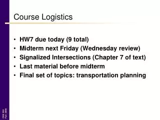
Course Logistics. HW7 due today (9 total) Midterm next Friday (Wednesday review) Signalized Intersections (Chapter 7 of text) Last material before midterm Final set of topics: transportation planning. Signalized Intersections. CEE 320 Anne Goodchild. Outline. Key Definitions

Course Logistics
E N D
Presentation Transcript
Course Logistics • HW7 due today (9 total) • Midterm next Friday (Wednesday review) • Signalized Intersections (Chapter 7 of text) • Last material before midterm • Final set of topics: transportation planning
Signalized Intersections CEE 320Anne Goodchild
Outline • Key Definitions • Baseline Assumptions • Control Delay • Signal Analysis • D/D/1 • Random Arrivals • LOS Calculation • Optimization
Key Definitions (1) • Cycle Length (C) • The total time for a signal to complete a cycle • Phase • The part of the signal cycle allocated to any combination of traffic movements receiving the ROW simultaneously during one or more intervals (a consistent period) • Green Time (G) • The duration of the green indication of a given movement at a signalized intersection • Red Time (R) • The period in the signal cycle during which, for a given phase or lane group, the signal is red
Key Definitions (2) • Change Interval (Y) • Yellow time • The period in the signal cycle during which, for a given phase or lane group, the signal is yellow • Clearance Interval (AR) • All red time • The period in the signal cycle during which all approaches have a red indication
Key Definitions (3) • Start-up Lost Time (l1) • Time used by the first few vehicles in a queue while reacting to the initiation of the green phase and accelerating. 2 seconds is typical. • Clearance Lost Time (l2) • Time between signal phases during which an intersection is not used by traffic. 2 seconds is typical. • Lost Time (tL) • Time when an intersection is not effectively used by any approach. 4 seconds is typical. • tL = l1 + l2
Key Definitions (4) • Effective Green Time (g) • Time effectively utilized for movement • g = G + Y + AR – tL • Effective Red Time (r) • Time during which a movement is effectively not permitted to move. • r = R + tL • r = C – g
C l2 l1 space AR end of intersection Green Red Yellow Red time G Y R saturation headway headways typically longer
Key Definitions (5) • Saturation Flow Rate (s) • Maximum flow that could pass through an intersection if 100% green time was allocated to that movement. • S (vehicles/hour) = 3600/headway (seconds per vehicle) • Approach Capacity (c) • Saturation flow times the proportion of effective green • c = s × g/C
Key Definitions (6) • Flow Ratio • The ratio of actual flow rate (v) to saturation flow rate (s) for a lane group at an intersection • Lane Group • A set of lanes established at an intersection approach for separate analysis • Critical Lane Group • The lane group that has the highest flow ratio (v/s) for a given signal phase • Critical Volume-to-Capacity Ratio (Xc) • The proportion of available intersection capacity used by vehicles in critical lane groups • In terms of v/c and NOT v/s
Baseline Assumptions • D/D/1 queuing • Approach arrivals < departure capacity • (no queue exists at the beginning/end of a cycle)
Quantifying Control Delay • Two approaches • Deterministic (uniform) arrivals (Use D/D/1) • Probabilistic (random) arrivals (Use empirical equations) • Total delay can be expressed as • Total delay in an hour (vehicle-hours, person-hours) • Average delay per vehicle (seconds per vehicle)
D/D/1 Signal Analysis (Graphical) Departure Rate Arrival Rate Vehicles Queue dissipation Total vehicle delay per cycle Maximum delay Maximum queue Time Green Green Red Red Green Red
D/D/1 Signal Analysis – Numerical • Time to queue dissipation after the start of effective green • Proportion of the cycle with a queue • Proportion of vehicles stopped
D/D/1 Signal Analysis – Numerical • Maximum number of vehicles in a queue • Total delay per cycle • Average vehicle delay per cycle • Maximum delay of any vehicle (assume FIFO)
Definition – Level of Service (LOS) • Chief measure of “quality of service” • Describes operational conditions within a traffic stream • Does not include safety • Different measures for different facilities • Six levels of service (A through F) • Based on control delay measure
Control Delay • Applies to both signalized and not signalized intersections • Referred to as signal delay for a signalized intersection • Total delay experienced by the driver as a result of the control • Includes deceleration time, queue move-up time, stop time, and acceleration time
Signal Analysis – Random Arrivals • Webster’s Formula (1958) - empirical d’ = avg. veh. delay assuming random arrivals d = avg. veh. delay assuming uniform arrivals (D/D/1) x = ratio of arrivals to departures (lc/mg) g = effective green time (sec) c = cycle length (sec)
Signal Analysis – Random Arrivals • Allsop’s Formula (1972) - empirical d’ = avg. veh delay assuming random arrivals d = avg. veh delay assuming uniform arrivals (D/D/1) x = ratio of arrivals to departures (lc/mg)
Signalized Intersection LOS • Based on control delay per vehicle • How long you wait, on average, at the stop light from Highway Capacity Manual 2000
Typical Approach • Split control delay into three parts • Part 1: Delay calculated assuming uniform arrivals (d1). This is essentially a D/D/1 analysis. • Part 2: Delay due to random arrivals (d2) • Part 3: Delay due to initial queue at start of analysis time period (d3).
Initial Queue Delay (d3) • Applied in cases where X > 1.0 for the analysis period • Vehicles arriving during the analysis period will experience an additional delay because there is already an existing queue • When no initial queue… • d3 = 0
Control Optimization • Conflicting Operational Objectives • minimize vehicle delay • Fuel consumption • Air quality • minimize vehicle stops • minimize lost time • major vs. minor service (progression) • pedestrian service • reduce accidents/severity
The “Art” of Signal Optimization • Long Cycle Length • High capacity (reduced lost time) • High delay on movements that are not served • Less efficient if uneven demand • Short Cycle Length • Reduced capacity (increased lost time) • Reduced delay for any given movement • More efficient if equal demand • “snappy” operations
Minimum cycle length • set Xc = 1.0 • critical v/c will be 1 • you can just squeeze all the vehicles through on that phase’s green time • However, if you set Xc = 1 • there will be times when more arrivals than your assumed v will show up and the cycle will fail • Therefore, often values less than 1 are assumed for Xc (such as 0.90).
Effective Width (WE) from Highway Capacity Manual 2000
Examples Signalized Intersections
Example SB At an intersection, saturation headways of 3 seconds are observed. What is the saturation flow rate? s=3600/3=1200 vehicles/hour WB EB NB
Example SB If GNB= 20 seconds, YNB= 3 seconds, RNB= 18 seconds, and AR= 2 seconds. What are the effective red and green times? The cycle time, and the lane-group capacity? g=20+3+2+4= 29 seconds r=18+4=22 seconds C=22+29=51 seconds c=1200*29/51=682 vehicles/hour WB EB NB
D/D/1 Signal Analysis (Graphical) Assumes g>C Departure Rate Arrival Rate Vehicles Queue dissipation Total vehicle delay per cycle Maximum delay Maximum queue Time Green Green Red Red Green Red
Determine total vehicle delay over 3 cycles if arrival rate is 500 veh/hr • Arrival rate: 500/3600=.139 veh/sec • Departure rate: 1200/3600=.333 vehicles/second • Traffic intensity = .139/.333 = .417 • Check capacity exceed arrivals: • .333x29=9.65 vehicles can get through on green • .139x51=7.09 vehicles arrive in cycle
Total vehicle delay • One cycle – 0.139*(22)2/2(1-.417)=57.5 vehicle seconds • Three cycles = 173 vehicle seconds
Example SB An intersection operates using a simple 3-phase design as pictured. WB EB NB
SB 150 30 400 30 EB 200 WB 300 20 1000 50 100 NB Example What is the sum of the flow ratios for the critical lane groups (Yc)? What is the total lost time for a signal cycle assuming 2 seconds of clearance lost time and 2 seconds of startup lost time per phase?
Key Definitions • Flow Ratio: The ratio of actual flow rate (v) to saturation flow rate (s) for a lane group • Critical Lane Group: The lane group that has the highest flow ratio (v/s) for a given signal phase • Volume to Capacity ratio (X): v/c or C/g • Critical Volume-to-Capacity Ratio (Xc): The proportion of available intersection capacity used by vehicles in critical lane groups • Sum of the Flow Ratios for the Critical Lane Groups (Yc): sum of flow ratios for critical lane groups
Example • PHASE 1: SB T/left/right= (400+150+30)/3400 = 0.171 • PHASE 2: NB T/left/right = (1000+100+50)/3400 = 0.338 • PHASE 3: • EB T/right = (200+20)/1400 = 0.157 • WB T/right = (300+30)/1400 = 0.236 limiting since v/s is highest • Yc=0.171 + 0.338 + 0.236 = 0.745 • Total lost time = 3(2+2) = 12 seconds
Example Calculate an optimal cycle length using Webster’s formula, and a minimum cycle length. Copt = 1.5(12 seconds) + 5/(1-0.745) = 90.2 seconds Cmin = (12 seconds) (0.9)/ (0.9-0.745) = 69.7 seconds
Minimum cycle length • set Xc = 1.0 • critical v/c will be 1 • you can just squeeze all the vehicles through on that phase’s green time • However, if you set Xc = 1 • there will be times when more arrivals than your assumed v will show up and the cycle will fail • Therefore, often values less than 1 are assumed for Xc (such as 0.90).
Example Determine the green times allocation (assume C=95 seconds)
DETERMINE Xc • Xc = 0.745(95)/(95 – 12) = 0.853 • CALCULATE EFFECTIVE GREEN TIMES • gSB = 0.171(95/0.853) = 19.04 seconds • gNB = 0.338(95/0.853) = 37.64 seconds • gEBWB = 0.236 (95/0.853) = 26.28 seconds • CHECK • 19.04 + 37.64 + 26.28 + 12 = 94.96 = 95 seconds
Example What is the intersection Level of Service (LOS)? Assume in all cases that PF = 1.0, k = 0.5 (pretimed intersection), I = 1.0 (no upstream signal effects).
Signalized Intersection LOS • Based on control delay per vehicle • How long you wait, on average, at the stop light from Highway Capacity Manual 2000
Typical Approach • Split control delay into three parts • Part 1: Delay calculated assuming uniform arrivals (d1). This is essentially a D/D/1 analysis. • Part 2: Delay due to random arrivals (d2) • Part 3: Delay due to initial queue at start of analysis time period (d3).