Statistical Techniques I
Statistical Techniques I. EXST7005. Sample Size Calculation. The sample size formula. The Z-test and t-test use a similar formula. . Lets suppose we know everything in the formula except n. Do we really? Maybe not, but we can get some pretty good estimates.

Statistical Techniques I
E N D
Presentation Transcript
Statistical Techniques I EXST7005 Sample Size Calculation
The sample size formula • The Z-test and t-test use a similar formula.
Lets suppose we know everything in the formula except n. Do we really? Maybe not, but we can get some pretty good estimates. • Call the numerator (`Y - m0) a difference, `d. It is some mean difference we want to be able to detect, so `d = `Y - m0. • The value s2 is a variance, the variance of the data that we will be sampling. We need this variance, or an estimate, S2. The sample size formula (continued)
The sample size formula (continued) • So we alter the formula to read.
The sample size formula (continued) • What other values do we know? Do we know Z? No, but we know what Z we need to obtain significance. If we are doing a 2-tailed test, and we set a = 0.05, then Z will be 1.96. • Any calculated value larger will be "more significant", any value smaller will not be significant. • So, if we want to detect significance at the 5% level, we can state that ...
The sample size formula (continued) • We will get a significant difference if
The sample size formula (continued) • We square both sides and solve for n. Then we will also get a significant difference if
The sample size formula (continued) • Then, if we have an idea of values for `d, s2, and Z, we can solve the formula for n. • If we are going to use a Z distribution we should have a known value of the variance (s2). If the variance is calculated from the sample, use the t distribution. • This would give us the sample size needed to obtain "significance", in accordance with whatever Z value is chosen.
Try an example where • `d = 2 • s2 = 5 • Z = 1.96 • So what value of n would detect this difference with this variance and produce a value of Z equal to 1.96 (or greater)? • n ³ (Z2s2)/`d2 = (1.962 * 52)/22 = 3.8416(25)/4 = 24.01 • since n ³ 24.01, round up to 25. Generic Example
Answer, n ³ 25 would produce significant results. • Guaranteed? • Wouldn't this always produce significant results? Theoretically, within the limits of statistical probability of error, yes. But only IF THE DIFFERENCE WAS REALLY 2. • If the null hypothesis (no difference,`Y-m0=0) was really true and we took larger samples, then we would get a better estimate of 0, and may never show significance. Generic Example (continued)
The formula we have seen contains only Za/2 or ta/2, depending on whether we have s2 or S2. However, a fuller version can contain consideration of the probability of Type II error (b). • Remember that to work with b we need to know the mean of the real distribution. However, in calculating sample size we have a difference,`d = `Y - m0. So we can include consideration of type II error. Considering Type II Error
Considering Type II Error (continued) • b error consideration would be done by adding another Z or t for the error rate. Notice that below I switch to t distributions and use S2.
Other examples • We have done a number of tests, some yielding significant results and others not. • If a test that yields significant results (showing a significant difference between the observed and hypothesized values), then we don't need to examine sample size because the sample was big enough. • However, some utility may be made of this information if we FAIL to reject the null hypothesis.
Recall the Rhesus monkey experiment. We hypothesized no effect of a drug, and with a sample size of 10 were unable to reject the null hypothesis. • However, we did observe a difference of +0.8 change in blood pressure after administering the drug. • What if this change was real? What if we made a Type II error? How large a sample would we need to test for a difference of 0.8 if we also wanted 90% power? An example with t values and b error included
An example with t values and b error included (continued) • So we want to know how large a sample we would need to get significance at the a=0.05 level if power was 0.90. In this case b=0.10. To do this calculation we need a two tailed a and a one tailed b (we know that the change is +0.8). • We will estimate the variance from the sample so we will use the t distribution. However, since we don't know the sample size we don't know the d.f.!
An example with t values and b error included (continued) • So we will approximate to start with. • Given the information, • a = 0.05 so t will be approximately 2 • b = 0.10 so t will be roughly 1.3 • `d =`Y-m0 = 0.8 from our previous results, and • S2 = 9.0667 from our previous results.
An example with t values and b error included (continued) • We do the calculations. • And now we have an estimate of n and the degrees of freedom. n = 155 and d.f.=154. We can refine our values for ta/2 and tb. • for d.f. = 154, ta/2 = 1.97 approx. • for d.f. = 154, tb = 1.287 approx.
An example with t values and b error included (continued) • So we redo the calculations with improved estimates. • A little improvement. If we saw much change in the estimate of n, we could recalculate as often as necessary. Usually 3 or 4 recalculations is enough.
We developed a formula for calculating sample size. • This formula can be adapted for either t or Z distributions. Summary
We learned that • We need input values of • a, • b, • S2 (or s2) • and we need to know what difference we want to detect (`d). Summary (continued)
Summary (continued) • We saw that for the t-test, the first calculation was only approximate since we didn't know the degrees of freedom and could not get the appropriate value of t. • However, after the initial calculation the estimate could be improved by iteratively recalculating the estimate of the value of n until it was stable.