Statistical Techniques I
Statistical Techniques I. EXST7005. Distribution of Sample Means. OBJECTIVES. Usually we will be testing hypotheses about means. We will need some additional information about the nature of means of samples in order to do hypothesis tests.

Statistical Techniques I
E N D
Presentation Transcript
Statistical Techniques I EXST7005 Distribution of Sample Means
OBJECTIVES • Usually we will be testing hypotheses about means. We will need some additional information about the nature of means of samples in order to do hypothesis tests.
Means are the basis for testing hypotheses about , the most common types of hypothesis tests. • Imagine a POPULATION from which we are drawing samples. • Population size = N • Mean = • Variance = 2 • Parent population values are: • Yi = Y1, Y2, Y3 , ... , YN Distribution of Sample Means
Distribution of Sample Means (continued) • The samples of size n form a DERIVED POPULATION • There are Nn possible samples of size n that can be drawn from a population of size N (sampling WITH replacement). • for each sample we calculate a mean • Yk = Yi/n • where k = 1, 2, 3, ... , Nn
Distribution of Sample Means (continued) • The Derived Population of Means of samples of size n • Population size = Nn • Mean = Y • Variance = Y • Derived population values • Yk = Y1, Y2, Y3, ... , YNn
Distribution of Sample Means (continued) • Mean of the DERIVED POPULATION • Y = Yk/Nn • where k = 1, 2, 3, ... , Nn • Variance of the DERIVED POPULATION • 2Y = Yk-)2/Nn • where k = 1, 2, 3, ... , Nn • n = the sample size • N = the population size • Population size = Nn
Original Population 0.25 r.f. 0.00 0 1 2 3 Example of a Derived Population • Parent Population: Yi = 0, 1, 2, 3 • = Yi/N = 6/4=1.5 • 2 = Yi-)2/N = [(0-1.5)2+(1-1.5)2+(2-1.5)2+(3-1.5)2]/4 = 5/4 = 1.25 • = 1.12
The Derived Population • The Derived Population • where n = 2 and • Nn = 42 = 16 • Draw all possible samples of size 2 from the Parent Population (sampling with replacement, so that values will occur more than once), and • calculate Y for each sample (Nn).
The Derived Population Mean 0, 0 0.0 Sample 0, 1 0.5 0, 2 1.0 0, 3 1.5 1, 0 0.5 1, 1 1.0 1, 2 1.5 1, 3 2.0 2, 0 1.0 2, 1 1.5 2, 2 2.0 2, 3 2.5 3, 0 1.5 3, 1 2.0 3, 2 2.5 3, 3 3.0
Means Frequency Relative Freq Frequency table of the Derived Population 0.0 1 0.0625 0.5 2 0.1250 1.0 3 0.1875 1.5 4 0.2500 2.0 3 0.1875 2.5 2 0.1250 3.0 1 0.0625 Sum = 16 1
0.30 0.25 0.20 0.15 0.10 0.05 0.00 0.0 0.5 1.0 1.5 2.0 2.5 3.0 Histogram of the Derived Population • Note that the derived population is shaped more like the normal distribution than the original population. Derived Population
0.25 r.f. 0.00 0 1 2 3 0.30 0.25 0.20 0.15 0.10 0.05 0.00 0.0 0.5 1.0 1.5 2.0 2.5 3.0 • Find P(1Y2) • For the original population, • P(1Y2)=0.5000 • For the derived population, • P(1Y2)=0.6250 Probability statement from the two distributions
THEOREM on the distribution of sample means • Given a population with mean and variance 2, if we draw all possible samples of size n (with replacement) from the population and calculateY, then the derived population of all possible sample means will have • Mean: Y = • Variance: Y = 2/n • Standard deviation: Y = /n = 2/n
THEOREM on the distribution of sample means (continued) • Notice that the variance and standard deviation of the mean have "n" in the denominator. As a result, the variance of the derived population becomes smaller as the sample size increases regardless of the value of the population variance.
CENTRAL LIMIT THEOREM • AS THE SAMPLE SIZE (n) INCREASES, THE DISTRIBUTION OF SAMPLE MEANS OF ALL POSSIBLE SAMPLES, OF A GIVEN SIZE FROM A GIVEN POPULATION, APPROACHES A NORMAL DISTRIBUTION IF THE VARIANCE IS FINITE. If the base distribution is normal, then the means are normal regardless of n.
Why is this important? (and it is very important!) • If we are more interested in the MEANS (and therefore the distribution of the means) than the original distribution, then normality is a more reasonable assumption. • Often, perhaps even USUALLY, we will be MORE INTERESTED in the MEANS of the DISTRIBUTION THAN IN THE DISTRIBUTIONS of the INDIVIDUALS. CENTRAL LIMIT THEOREM (continued)
NOTES on the distribution of sample means • as n increases, Y and Y decrease. • Y for any n • Y for any n > 1 • as n increases and Y becomes smaller, the distribution of Y's becomes closer to Y. (i.e. we get a better estimate).
Some new terms • Reliability (as a statistical concept) - the closer the estimate of to the actual value of , the more "reliable" the estimate. • Accuracy (as a statistical concept) - this term refers to the lack of bias in the estimate, and not how small the variance is. An estimate may be very accurate, but have a great deal of scatter about the mean.
In practice we cannot draw all possible samples. • Recall that E(S2) = • so, S2Y = S2/n is an estimate of Y • where; • E(S2Y) = Y • and; • S2Y is an estimate of the variance of sample means of size n • S2 is the estimate of the variance of observations Estimation of Y and Y
Estimation of Y and Y (continued) • S2Y = S2/n is called the STANDARD ERROR to distinguish it from the Standard deviation • it is also called the Standard Deviation OF THE MEANS • NOTE: that this division is by "n" for both populations and samples, not by "n-1" as with the calculation of variance for samples.
Estimation of Y and Y (continued) • S2Y is a measure of RELIABILITY of the sample means as an estimate of the true population mean. • i.e. the smaller S2Y , the more reliableY as an estimate of • Ways of increasing RELIABILITY • Basically, anything that decreases our estimate of Y makes our estimate more reliable.
Estimation of Y and Y (continued) • How do we decrease our estimate of Y? • Increase the sample size; if n increases then Y decreases. • Decrease the variance; if our estimate of decreases then Y decreases. • This can sometimes be done by; • refining our measurement techniques • finding a more homogeneous population to measure
The Z transformation for a DERIVED POPULATION • We will use the Z transformation for two purposes, individuals and means. • for individuals use • Zi = (Yi - )/ • for means we will use • Zi = (Yi - Y)/Y
Summary • Most testing of hypotheses will concern tests of a derived population of means. • The mean of the derived population of sample means is Y • The Variance of the derived population of sample means is Y
Summary (continued) • The CENTRAL LIMIT THEOREM is an important aspect of hypothesis testing because it states that sample means tend to be more nearly normally distributed than the parent population. • Reliability and accuracy are statistical concepts relating to variability and lack of bias, respectively.