Figure 8.3 : Examples for variation types
Figure 8.1. Engineering drawing of the “steer support”, a critical component of the Xootr scooter. The “height” of the steer support is specified by the dimensions (shown in the lower center portion of the drawing) as falling between 79.900 and 80.000 mm.
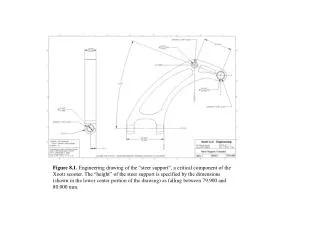

Figure 8.3 : Examples for variation types
E N D
Presentation Transcript
Figure 8.1. Engineering drawing of the “steer support”, a critical component of the Xootr scooter. The “height” of the steer support is specified by the dimensions (shown in the lower center portion of the drawing) as falling between 79.900 and 80.000 mm.
Figure 8.2. Steer support within Xootr scooter assembly. The height of the steer support must closely match the opening in the lower handle.
Process Parameter Upper Control Limit (UCL) Center Line Lower Control Limit (LCL) Time periods Figure 8.4: A generic control chart
12 10 8 6 X-Bar 4 2 0 1 3 5 7 9 11 13 15 17 19 21 23 25 27 30 25 20 15 R 10 5 0 1 3 5 7 9 11 13 15 17 19 21 23 25 27 Figure 8.6: Control charts for the An-ser case
Upper Specification Limit (USL) Lower Specification Limit (LSL) Process A (with st. dev sA) 3 Process B (with st. dev sB) X-3sA X-2sA X-1sA X X+1sA X+2s X+3sA X-6sB X X+6sB Figure 8.7: Comparison of three sigma and six sigma process capability
100 75 50 25 100 50 Number ofdefects Cumulativepercents ofdefects Browser error Order entrymistake Wrong modelshipped Order number out off sequence Product shipped tobilling address Product shipped, butcredit card not billed Figure 8.8: Order entry mistakes at Xootr
Step 1 Test 1 Step 2 Test 2 Step 3 Test 3 Rework Step 1 Test 1 Step 2 Test 2 Step 3 Test 3 Figure 8.9: Two processes with rework
Final Test Step 1 Step 2 Step 3 Step 1 Test 1 Step 2 Test 2 Step 3 Test 3 Figure 8.10: Process with scrap
End of Process Process Step Market Bottleneck Defectoccurred Defectdetected Defectdetected Defectdetected Defectdetected $ $ $ Cost of defect Based on labor andmaterial cost Based on salesprice (incl. Margin) Recall, reputation,warranty costs Figure 8.11.: Cost of a defect as a function of its detection location assuming a capacity constrained process
8 7 4 3 Defective unit 3 1 2 1 2 6 5 4 Good unit ITAT=7*1 minute ITAT=2*1 minute Figure 8.12.: Information turnaround time and its relationship with buffer size
Direction of production flow upstream downstream Authorize productionof next unit Figure 8.13.: Simplified mechanics of a Kanban system Kanban Kanban Kanban Kanban
Buffer argument:“Increase inventory” Inventory in process Toyota argument:“Decrease inventory” Figure 8.14.: More or less inventory? A simple metaphor
Flow Rate High Increase inventory(smooth flow) Path advocated byToyota production system Now Reduce inventory(blocking or starvingbecome more likely) New frontier Frontier reflecting current process Low High Inventory (Long ITAT) Low Inventory (short ITAT) Inventory Figure 8.15.: Tension between flow rate and inventory levels / ITAT