Download
1 / 54
550 likes | 1.24k Vues
Severity Distributions for GLMs: Gamma or Lognormal?. Presented by Luyang Fu, Grange Mutual Richard Moncher, Bristol West 2004 CAS Spring Meeting Colorado Springs, Colorado May 18, 2004. Session Outline. Introduction Distribution Assumptions Simulation Method Simulation Results

E N D
Severity Distributions for GLMs: Gamma or Lognormal? Presented by Luyang Fu, Grange Mutual Richard Moncher, Bristol West 2004 CAS Spring Meeting Colorado Springs, Colorado May 18, 2004
Session Outline • Introduction • Distribution Assumptions • Simulation Method • Simulation Results • Conclusions
Introduction • Common characteristics of loss distributions • Typical GLM forms in actuarial practice • Lognormal and Gamma are most widely-used distributions in size of loss (severity) analysis • Lognormal or Gamma?
Distribution Characteristics of Insurance Losses • Non-negative • Positively skewed • Variance is positively correlated with mean. • Normal is not appropriate: negative, symmetric, constant variance
Advantages of GLMs • Exponential Distribution Selections: Poisson, Gamma, Binomial, Inverse Gaussian, Negative Binomial, etc. Lognormal is not in exponential family. • Link Function Selections: Identity, Log, Logit, Power, Probit, etc.
Typical GLM Forms in Actuarial Practice • Severity: Log link, Gamma Distribution • Frequency: Log link, Poisson Distribution • Retention (Renewal): Logit link, Binomial Distribution
Gamma or Lognormal? • Gamma and lognormal are the two most popular selections of loss distributions • On CAS website (www.casact.org), we found 31 papers by searching “Lognormal” and 37 papers by searching “Gamma”
Lognormal Is One of Most Widely-Used Loss Distributions Proceedings of the Casualty Actuarial Society • Ratemaking and Reinsurance Wacek, Michael G.(1997) Bear, Robert A.; Nemlick, Kenneth J. (1990) Hayne, Roger M. (1985) Mack, Thomas (1984) Ter Berg, Peter (1980) Benckert, Lars-Gunnar (1962)
Lognormal Is One of Most Widely-Used Loss Distributions Proceedings of the Casualty Actuarial Society • Reserving and Reinsurance Kreps, Rodney E. (1997) Ramsay, Colin M.; Usabel, Miguel A. (1997) Doray, Louis G. (1996) Levi, Charles; Partratm, Christian (1991) Hertig, Joakim (1985)
Lognormal Is One of Most Widely-Used Loss Distributions • In actuarial practice Increased Limit Factors Excess of Loss Calculations Weather Load Quantile Loss Reserve Variability
Gamma or Lognormal? • Desirable Features of Gamma and Lognormal Distributions: 1. Non-negative 2. Positively skewed 3. Variance is proportional to the mean-squared (Constant Coefficient of Variation)
Gammaor Lognormal? Advantages of Lognormal: • Easy to understand (related to normal distribution) • Consistent with other actuarial procedures, such as increased limits ratemaking • Fits data with large skewness well Disadvantage of Lognormal: • Not in exponential family, and GLM coefficients need volatility adjustment
Gamma or Lognormal? • Under what conditions are the severity distribution assumptions important? • If severity distribution is unknown, which distribution yields most accurate and stable results (i.e., minimized estimation bias and standard error)?
Classical Distribution Assumptions • Normal Constant Variance • Gamma Constant Coefficient of Variation
Classical Distribution Assumptions • Lognormal Constant Coefficient of Variation
Does Normal Necessarily Imply Constant Variance? • Normal Constant Coefficient of Variation: Variance function is like Gamma • Normal Variance proportional to mean: Variance function is like Poisson
Does Gamma Necessarily Imply Constant Coefficient of Variation? • Gamma Variance is proportional to mean: Variance function is like Poisson.
Distribution Assumptions • One of two parameters is constant • Which one is selected as constant should be based on data • Classical assumptions are most-widely used distribution forms, and generally fit data better • Can we assume none of them are constant? Yes, but it will increase the number of parameters and reduce the degrees of freedom
Why Simulation? • The distributions of GLM coefficients and predicted values are unknown in the case of small samples • Statistical analysis based on asymptotic distributions is not reliable • In an individual regression, we don’t know if the difference between predicted value and observed value is from random variation or systematic bias
Simulation Assumptions • 32 Severity Observations for Two Class Variables • 8 Age Groups • 4 Vehicle-Use Groups • Data Source: Private Passenger Auto Collision used in Mildenhall (1999) and McCullagh and Nelder (1989)
Simulation Assumptions • Individual Losses Have Constant Coefficient of Variation • Multiplicative Relationship Between Severities and Rating Variables • Known “True” Base Severities & Relativities • Known CVs for the Severity Distribution
Simulation Procedures • Generate individual losses based on lognormal and gamma distributions and calculate 32 claim severities • Fit three regressions: GLM with Gamma, GLM with Normal, and GLM with log-transformed severity • Repeat Steps 1-2 one thousand times, and generate sampling distributions of GLM coefficients and predicted values
Performance Measurements • Weighted Absolute Bias, which measures the systematic bias (accuracy): • Weighted Standard Error, which measures random variation (stability):
Adjustments for Log-Transformed Regressions • GLMs with Gamma and Normal • Log-transformed Regression is called the “Volatility Adjustment Factor”
Simulation Results • Data Generated • Regression Results • Residual Diagnostics
Data Generated Reporting on Two Different Classes: • Classification I - Age 17-20 and Pleasure Use, with 21 observations. • Classification II - Age 40-49 and Short Drive to Work, with 970 observations.
Data Generated: Gamma Severity for Age 17-20 and Pleasure Use with Coefficient of Variation 3.0
Data Generated: Gamma Severity for Age 40-49 and DTW Short Use with Coefficient of Variation 3.0
Data Generated: Lognormal Severity for Age 17-20 and Pleasure Use with Coefficient of Variation 3.0
Data Generated: Lognormal Severity for Age 40-49 and DTW Short Use with Coefficient of Variation 3.0
CV wab wse G-G G-L G-N G-G G-L G-N 1.0 0.180 0.240 0.221 8.170 8.177 8.568 2.0 0.475 0.852 0.509 16.498 16.514 17.239 3.0 0.860 1.808 1.139 25.223 25.097 26.986 Regression Results Overall Unbiasedness and Stability of Predicted Severities for Gamma Loss
CV wab wse L-G L-L L-N L-G L-L L-N 1.0 0.151 0.202 0.175 8.309 8.284 8.754 2.0 0.498 0.844 0.604 16.426 16.113 17.721 3.0 0.720 1.589 1.006 24.328 23.214 27.608 Regression Results Overall Unbiasedness and Stability of Predicted Severities for Lognormal Loss
Regression Results: Predicted Severities for Gamma Loss with Coefficient of Variation 3.0 for Age 17-20 and Pleasure Use
Regression Results: Predicted Severities for Gamma Loss with Coefficient of Variation 3.0 for Age 40-49 and DTW Short Use
Regression Results: Predicted Severities for Lognormal Loss with Coefficient of Variation 3.0 for Age 17-20 and Pleasure Use
Regression Results: Predicted Severities for Lognormal Loss with Coefficient of Variation 3.0 for Age 40-49 and DTW Short Use
Residual Diagnostics: Standardized Residuals for Gamma Loss with Coefficient of Variation 3.0
Residual Diagnostics: Predicted Severities vs Standardized Residuals for Gamma Loss with Coefficient of Variation 3.0
Residual Diagnostics: Standardized Residuals for Lognormal Loss with Coefficient of Variation 3.0
Residual Diagnostics: Predicted Severities vs Standardized Residuals for Lognormal Loss with Coefficient of Variation 3.0
Residual Diagnostics: Standardized Residuals for Gamma Loss with Coefficient of Variation 1.0 Based on Individual Data
Residual Diagnostics: Predicted Severities vs Standardized Residuals for Gamma Loss with Coefficient of Variation 1.0 Based on Individual Data
Residual Diagnostics: Standardized Residuals for Lognormal Loss with Coefficient of Variation 1.0 Based on Individual Data
Residual Diagnostics: Predicted Severities vs Standardized Residuals for Lognormal Loss with Coefficient of Variation 1.0 Based on Individual Data
Conclusions • When the gamma distribution is “true”, the G-G model is dominant in both unbiasedness and stability (except the G-L model is slightly more stable in the case of large volatility).
Conclusions • When the lognormal distribution is “true”, the L-L model is dominant in terms of stability.
Conclusions • GLMs with a normal distribution never dominate based on any criteria, and they have the worst weighted standard error.
Conclusions • GLMs with a gamma distribution are dominant in terms of unbiasedness, no matter whether the “true” distribution is gamma or lognormal.
Conclusions • In general, GLMs with a gamma distribution are recommended because they perform slightly better than the log-transformed model.
Conclusions • When the data is not volatile, the distribution selection for GLMs may not be as important because all distribution assumptions yield small biases and standard errors.