Rainfall-Runoff Modeling (2)
Rainfall-Runoff Modeling (2). Professor Ke-Sheng Cheng Dept. of Bioenvironmental Systems Engineering National Taiwan University. Peak flow estimation. Rational method Empirical method Unit hydrograph technique. The concept of Isochrones.

Rainfall-Runoff Modeling (2)
E N D
Presentation Transcript
Rainfall-Runoff Modeling (2) Professor Ke-Sheng Cheng Dept. of Bioenvironmental Systems Engineering National Taiwan University
Peak flow estimation • Rational method • Empirical method • Unit hydrograph technique
The concept of Isochrones • Let’s assume that raindrops fall on a spatial point x within the watershed require an amount of travel timet(x) to move from point x to the basin outlet.
Contour lines of the travel time are termed as isochrones (or runoff isochrones) of the watershed. • The highest value of isochrones represents the time of concentration of the watershed. • Assume the effective rainfall has a constant intensity (in time) and is uniformly distributed over the whole watershed, i.e.,
If the effective rainfall duration tr = 2 hours, what is the peak direct runoff at the basin outlet? When will the peak flow occur? When will the direct runoff end?
The time of peak flow occurrence is dependent on the relative magnitude of Ai’s.
If the effective rainfall duration tr = 10 hours, what is the peak direct runoff at the basin outlet? When will the peak flow occur? When will the direct runoff end?
Under the assumptions of constant intensity and uniform spatial distribution for effective rainfall, the peak direct runoff occurs at the time t = tc, if the duration of the effective rainfall is longer than or equal to tc.
However, for storms with duration shorter than tc, the peak flow and its time of occurrence depend on relative magnitude of contributing areas (Ai’s).
Rational method for peak flow estimation • Consider a rainfall of constant intensity and very long duration occurring uniformly over a basin. The runoff gradually increases from zero to a constant value as shown in the following figure.
Practical application of the rational method for peak flow estimation • Calculating the time of concentration, tc. • Determining the average rainfall intensity i from the IDF curve using tc as the storm duration and a predetermined return period T. • Calculating the runoff coefficient, c. • Calculating the peak direct runoff In engineering practice, it is normally restricted to catchments with basin area not exceeding 15 km2.
Unit hydrograph of the modified rational method tc+tr 2tc Neglecting the watershed storage effect. • Original rational method only estimates the peak flow. It does not yield the complete runoff hydrograph.
Synthetic unit hydrographs • For areas where rainfall and runoff data are not available, unit hydrograph can be developed based on physical characteristics of the watershed. • Clark’s IUH (time-area method) • SCS unit hydrograph • Linear reservoir model (Nash model)
Clark’s IUH (time-area method) • The concept of isochrones • Isochrones are lines of equal travel time. Any point on a given isochrone takes the same time to reach the basin outlet. Therefore, for the following basin isochrone map and assuming constant and uniform effective rainfall, discharge at the basin outlet can be decomposed into individual contributing areas and rainfalls.
Using the basin isochrone map, the cumulative contributing area curve can be developed. The derivatives or differences of this curve constitute the instantaneous unit hydrograph IUH(t). Time base of the IUH is the time of concentration of the watershed.
If the effect of watershed storage is to be considered, the unit hydrograph described above is routed through a hypothetical linear reservoir with a storage coefficient k located at the watershed outlet. • For a linear reservoir with storage coefficient k, we have
Consider the continuity of the hypothetical reservoir during a time interval t.
Example. A watershed of 1000-acre drainage area has the following 15-minute time-area curve. The storage coefficient k of the watershed is 30 minutes. Determine the 15-minute unit hydrograph UH(15,t).
Area between isochrones t = 0 and t = 0.25 hr is 100 acres. Since we are interested in the unit hydrograph UH(15-min, t), the rainfall intensity in the time period (0.25 hr) should be 4 inch/hr. Therefore, the ordinate of UH(15-min, t) at time t = 0.25 hr is: 4 inch/hr (1/12 ft/inch) (1/3600 hr/sec) 100 acres (43560 ft2/acre) = 403.33 cfs
Synthetic unit hydrographs • Clark’s IUH (time-area method) • SCS unit hydrograph • Linear reservoir model (Nash model)
SCS unit hydrograph Note: tb > tr+tc. The SCS UH takes into account the storage effect.
tc=0.5 Misuse of SCS UH – an example
Synthetic unit hydrographs • Clark’s IUH (time-area method) • SCS unit hydrograph • Linear reservoir model (Nash model)
Nash’s linear reservoir model • Consider a linear reservoir which has the following characteristics:
Summary of the Conceptual IUH modelAssumption: Linear Reservoir S(t)=kQ(t)
The above equation represents a gamma density function, and thus the integration over 0 to infinity yields 1 (one unit of rainfall excess).
=M1 =M2 Parameter estimation for n and k • The IUH of the n-LR system is characterized by a function which is identical to the gamma density.
The direct runoff can be expressed as a convolution integral of the rainfall excess and IUH, i.e. • If the direct runoff hydrograph (DRH) is divided by the total volume of direct runoff, it can be viewed as a density function. Thus, denotes a density function of a random variable t. • The first moment of this rescaled DRH is
The second moment of the rescaled DRH is • Similarly, the first and second moments of the rescaled effective rainfall can be respectively expressed as