Interest Points
10/24/13. Interest Points. Computational Photography Derek Hoiem, University of Illinois. Galatea of the Spheres Salvador Dali. Today’s class. Review of “Modeling the Physical World” Interest points. Vote for project 3 favorites!. Pinhole camera model. Linear projection from 3D to 2D

Interest Points
E N D
Presentation Transcript
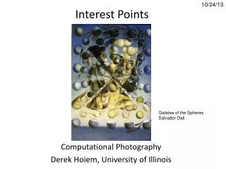
10/24/13 Interest Points Computational Photography Derek Hoiem, University of Illinois Galatea of the Spheres Salvador Dali
Today’s class • Review of “Modeling the Physical World” • Interest points
Pinhole camera model • Linear projection from 3D to 2D • Be familiar with projection matrix (focal length, principal point, etc.) . Optical Center (u0, v0) . . f Z Y v . Camera Center (tx, ty, tz) u
Vanishing points and metrology 5 Vertical vanishing point (at infinity) 4 3 Vanishing line 2 1 Vanishing point Vanishing point • Parallel lines in 3D intersect at a vanishing point in the image • Can measure relative object heights using vanishing point tricks
Single-view 3D Reconstruction • Technically impossible to go from 2D to 3D, but we can do it with simplifying models • Need some interaction or recognition algorithms • Uses basic VP tricks and projective geometry
Lens, aperture, focal length • Aperture size and focal length control amount of exposure needed, depth of field, field of view Good explanation: http://www.cambridgeincolour.com/tutorials/depth-of-field.htm
One small snag • How do we deal with light sources? Sun, lights, etc? • They are much, much brighter than the rest of the environment • Use High Dynamic Range photography! Relative Brightness . 1907 . 46 . 15116 . 1 . 18
Key ideas for Image-based Lighting • Capturing HDR images: needed so that light probes capture full range of radiance
Key ideas for Image-based Lighting • Relighting: environment map acts as light source, substituting for distant scene
Next section of topics • Correspondence • How do we find matching patches in two images? • How can we automatically align two images of the same scene? • How do we find images with similar content? • How do we tell if two pictures are of the same person’s face? • How can we detect objects from a particular category? • Applications • Photo stitching • Object recognition • 3D Reconstruction
How can we align two pictures? • Case of global transformation
How can we align two pictures? • Global matching? • But what if • Not just translation change, but rotation and scale? • Only small pieces of the pictures match?
Today: Keypoint Matching 1. Find a set of distinctive key- points 2. Define a region around each keypoint A1 B3 3. Extract and normalize the region content A2 A3 B2 B1 4. Compute a local descriptor from the normalized region 5. Match local descriptors K. Grauman, B. Leibe
Question • Why not just take every patch in the original image and find best match in second image?
Goals for Keypoints Detect points that are repeatable and distinctive
Key trade-offs B3 A1 A2 A3 B2 B1 Localization More Repeatable More Points Robust to occlusion Works with less texture Robust detection Precise localization Description More Selective More Robust Minimize wrong matches Deal with expected variations Maximize correct matches
Keypoint localization original • Suppose you have to click on some point, go away and come back after I deform the image, and click on the same points again. • Which points would you choose? deformed
Choosing interest points Where would you tell your friend to meet you?
Choosing interest points Where would you tell your friend to meet you?
Choosing interest points • Corners • Peaks/Valleys
Many Existing Detectors Available Hessian & Harris [Beaudet ‘78], [Harris ‘88] Laplacian, DoG[Lindeberg ‘98], [Lowe 1999] Harris-/Hessian-Laplace [Mikolajczyk & Schmid ‘01] Harris-/Hessian-Affine [Mikolajczyk & Schmid ‘04] EBR and IBR [Tuytelaars & Van Gool ‘04] MSER[Matas ‘02] Salient Regions [Kadir & Brady ‘01] Others… K. Grauman, B. Leibe
Harris Detector [Harris88] Second moment matrix Intuition: Search for local neighborhoods where the image gradient has two main directions (eigenvectors). K. Grauman, B. Leibe
Ix Iy Harris Detector [Harris88] • Second moment matrix 1. Image derivatives Iy2 IxIy Ix2 2. Square of derivatives g(IxIy) g(Ix2) g(Iy2) 3. Gaussian filter g(sI) 4. Cornerness function – both eigenvalues are strong g(IxIy) 5. Non-maxima suppression har
Matlab code for Harris Detector function [ptx, pty] = detectKeypoints(im, alpha, N) % get harris function gfil= fspecial('gaussian', [7 7], 1); % smoothing filter imblur = imfilter(im, gfil); % smooth image [Ix, Iy] = gradient(imblur); % compute gradient Ixx = imfilter(Ix.*Ix, gfil); % compute smoothed x-gradient sq Iyy = imfilter(Iy.*Iy, gfil); % compute smoothed y-gradient sq Ixy= imfilter(Ix.*Iy, gfil); har= Ixx.*Iyy - Ixy.*Ixy - alpha*(Ixx+Iyy).^2; % cornerness % get local maxima within 7x7 window maxv = ordfilt2(har, 49, ones(7)); % sorts values in each window maxv2 = ordfilt2(har, 48, ones(7)); ind = find(maxv==har & maxv~=maxv2); % get top N points [sv, sind] = sort(har(ind), 'descend'); sind = ind(sind); [pty, ptx] = ind2sub(size(im), sind(1:min(N, numel(sind))));
Harris Detector – Responses [Harris88] Effect: A very precise corner detector.
Automatic Scale Selection How to find corresponding patch sizes? K. Grauman, B. Leibe
Automatic Scale Selection • Function responses for increasing scale (scale signature) K. Grauman, B. Leibe
Automatic Scale Selection • Function responses for increasing scale (scale signature) K. Grauman, B. Leibe
Automatic Scale Selection • Function responses for increasing scale (scale signature) K. Grauman, B. Leibe
Automatic Scale Selection • Function responses for increasing scale (scale signature) K. Grauman, B. Leibe
Automatic Scale Selection • Function responses for increasing scale (scale signature) K. Grauman, B. Leibe
Automatic Scale Selection • Function responses for increasing scale (scale signature) K. Grauman, B. Leibe
What Is A Useful Signature Function? • Difference of Gaussian = “blob” detector K. Grauman, B. Leibe
Difference-of-Gaussian (DoG) = - K. Grauman, B. Leibe
DoG – Efficient Computation • Computation in Gaussian scale pyramid Sampling withstep s4=2 s s s s Original image K. Grauman, B. Leibe
Results: Lowe’s DoG K. Grauman, B. Leibe
Orientation Normalization p 2 0 • Compute orientation histogram • Select dominant orientation • Normalize: rotate to fixed orientation [Lowe, SIFT, 1999] T. Tuytelaars, B. Leibe
Available at a web site near you… • For most local feature detectors, executables are available online: • http://robots.ox.ac.uk/~vgg/research/affine • http://www.cs.ubc.ca/~lowe/keypoints/ • http://www.vision.ee.ethz.ch/~surf K. Grauman, B. Leibe
Local Descriptors • The ideal descriptor should be • Robust • Distinctive • Compact • Efficient • Most available descriptors focus on edge/gradient information • Capture texture information • Color rarely used K. Grauman, B. Leibe
Local Descriptors: SIFT Descriptor • Histogram of oriented gradients • Captures important texture information • Robust to small translations / affine deformations [Lowe, ICCV 1999] K. Grauman, B. Leibe
Details of Lowe’s SIFT algorithm • Run DoG detector • Find maxima in location/scale space • Remove edge points • Find all major orientations • Bin orientations into 36 bin histogram • Weight by gradient magnitude • Weight by distance to center (Gaussian-weighted mean) • Return orientations within 0.8 of peak • Use parabola for better orientation fit • For each (x,y,scale,orientation), create descriptor: • Sample 16x16 gradient mag. and rel. orientation • Bin 4x4 samples into 4x4 histograms • Threshold values to max of 0.2, divide by L2 norm • Final descriptor: 4x4x8 normalized histograms Lowe IJCV 2004
Matching SIFT Descriptors • Nearest neighbor (Euclidean distance) • Threshold ratio of nearest to 2nd nearest descriptor Lowe IJCV 2004
Local Descriptors: SURF • Fast approximation of SIFT idea • Efficient computation by 2D box filters & integral images 6 times faster than SIFT • Equivalent quality for object identification • GPU implementation available • Feature extraction @ 200Hz(detector + descriptor, 640×480 img) • http://www.vision.ee.ethz.ch/~surf [Bay, ECCV’06], [Cornelis, CVGPU’08] K. Grauman, B. Leibe
What to use when? Detectors • Harris gives very precise localization but doesn’t predict scale • Good for some tracking applications • DOG (difference of Gaussian) provides ok localization and scale • Good for multi-scale or long-range matching Descriptors • SIFT: good general purpose descriptor

