Interest Points II
Interest Points II. TODAY : Invariant Features, SIFT Recap: Interest Points and Descriptors Harris, Correlation Image Sampling Scaling, rotation SIFT (scale invariant feature transform) Both interest point detector (DOG)… …and descriptor. Interest Points and Descriptors.
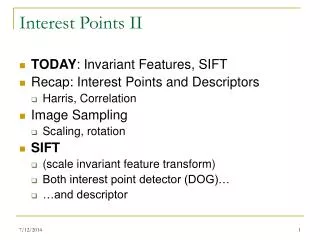

Interest Points II
E N D
Presentation Transcript
Interest Points II • TODAY: Invariant Features, SIFT • Recap: Interest Points and Descriptors • Harris, Correlation • Image Sampling • Scaling, rotation • SIFT • (scale invariant feature transform) • Both interest point detector (DOG)… • …and descriptor
Interest Points and Descriptors • Interest Points • Focus attention for image understanding • Points with 2D structure in the image • Examples: Harris corners, DOG maxima • Descriptors • Describe region around an interest point • Must be invariant under • Geometric distortion • Photometric changes • Examples: Oriented patches, SIFT
Image Sampling : Scale This is aliasing!
Y V 1 ? ? U ? ? θ X 1 Image Sampling : Rotation • Recall formula for 2D rotation: • Given a 2D grid of x, y pixel values… • what are the u, v pixel values?
Image Sampling : Rotation • Problem: sample grids are not aligned… X, Y U, V
y ? ? I x ? ? ? ? I x 1 Linear Interpolation • Find value between pixel samples I2 I01 I00 I11 I1 I10
Bilinear Interpolation • Use all 4 adjacent samples I01 I11 y I00 I10 x
The SIFT (Scale Invariant Feature Transform) Detector and Descriptor developed by David Lowe University of British Columbia Initial paper 1999 Newer journal paper 2004
Motivation • The Harris operator is not invariant to scale and its descriptor was not invariant to rotation1. • For better image matching, Lowe’s goal was to develop an operator that is invariant to scale and rotation. • The operator he developed is both a detector and a descriptor and can be used for both image matching and object recognition. 1But Schmid and Mohr developed a rotation invariant descriptor for it in 1997.
Idea of SIFT • Image content is transformed into local feature coordinates that are invariant to translation, rotation, scale, and other imaging parameters SIFT Features
Claimed Advantages of SIFT • Locality: features are local, so robust to occlusion and clutter (no prior segmentation) • Distinctiveness: individual features can be matched to a large database of objects • Quantity: many features can be generated for even small objects • Efficiency: close to real-time performance • Extensibility: can easily be extended to wide range of differing feature types, with each adding robustness
Overall Procedure at a High Level • Scale-space extrema detection • Keypoint localization • Orientation assignment • Keypoint description Search over multiple scales and image locations. Fit a model to detrmine location and scale. Select keypoints based on a measure of stability. Compute best orientation(s) for each keypoint region. Use local image gradients at selected scale and rotation to describe each keypoint region.
1. Scale-space extrema detection • Goal: Identify locations and scales that can be repeatably assigned under different views of the same scene or object. • Method: search for stable features across multiple scales using a continuous function of scale. • Prior work has shown that under a variety of assumptions, the best function is a Gaussian function. • The scale space of an image is a function L(x,y,) that is produced from the convolution of a Gaussian kernel (at different scales) with the input image.
Aside: Image Pyramids And so on. 3rd level is derived from the 2nd level according to the same funtion 2nd level is derived from the original image according to some function Bottom level is the original image.
Aside: Mean Pyramid And so on. At 3rd level, each pixel is the mean of 4 pixels in the 2nd level. At 2nd level, each pixel is the mean of 4 pixels in the original image. mean Bottom level is the original image.
Aside: Gaussian PyramidAt each level, image is smoothed and reduced in size. And so on. At 2nd level, each pixel is the result of applying a Gaussian mask to the first level and then subsampling to reduce the size. Apply Gaussian filter Bottom level is the original image.
Example: Subsampling with Gaussian pre-filtering G 1/8 G 1/4 Gaussian 1/2
Lowe’s Scale-space Interest Points • Laplacian of Gaussian kernel • Scale normalised (x by scale2) • Proposed by Lindeberg • Scale-space detection • Find local maxima across scale/space • A good “blob” detector
Lowe’s Scale-space Interest Points • Gaussian is an ad hoc solution of heat diffusion equation • Hence • k is not necessarily very small in practice
Lowe’s Scale-space Interest Points • Scale-space function L • Gaussian convolution • Difference of Gaussian kernel is a close approximate to scale-normalized Laplacian of Gaussian • Can approximate the Laplacian of Gaussian kernel with a difference of separable convolutions where is the width of the Gaussian. 2 scales: and k
Lowe’s Pyramid Scheme • Scale space is separated into octaves: • Octave 1 uses scale • Octave 2 uses scale 2 • etc. • In each octave, the initial image is repeatedly convolved • with Gaussians to produce a set of scale space images. • Adjacent Gaussians are subtracted to produce the DOG • After each octave, the Gaussian image is down-sampled • by a factor of 2 to produce an image ¼ the size to start • the next level.
Lowe’s Pyramid Scheme s+2 filters s+1=2(s+1)/s0 . . i=2i/s0 . . 2=22/s0 1=21/s0 0 s+2 differ- ence images s+3 images including original The parameter s determines the number of images per octave.
Key point localization s+2 difference images. top and bottom ignored. s planes searched. • Detect maxima and minima of difference-of-Gaussian in scale space • Each point is compared to its 8 neighbors in the current image and 9 neighbors each in the scales above and below For each max or min found, output is the location and the scale.
Scale-space extrema detection: experimental results over 32 images that were synthetically transformed and noise added. % detected % correctly matched average no. detected average no. matched Expense Stability • Sampling in scale for efficiency • How many scales should be used per octave? S=? • More scales evaluated, more keypoints found • S < 3, stable keypoints increased too • S > 3, stable keypoints decreased • S = 3, maximum stable keypoints found
2. Keypoint localization • Detailed keypoint determination • Sub-pixel and sub-scale location scale determination • Ratio of principal curvature to reject edges and flats (like detecting corners)
Keypoint localization • Once a keypoint candidate is found, perform a detailed fit to nearby data to determine • location, scale, and ratio of principal curvatures • In initial work keypoints were found at location and scale of a central sample point. • In newer work, they fit a 3D quadratic function to improve interpolation accuracy. • The Hessian matrix was used to eliminate edge responses.
Eliminating the Edge Response • Reject flats: • < 0.03 • Reject edges: • r < 10 • What does this look like? Let be the eigenvalue with larger magnitude and the smaller. Let r = /. So = r (r+1)2/r is at a min when the 2 eigenvalues are equal.
3. Orientation assignment • Create histogram of local gradient directions at selected scale • Assign canonical orientation at peak of smoothed histogram • Each key specifies stable 2D coordinates (x, y, scale,orientation) If 2 major orientations, use both.
Keypoint localization with orientation 832 233x189 initial keypoints 536 729 keypoints after ratio threshold keypoints after gradient threshold
4. Keypoint Descriptors • At this point, each keypoint has • location • scale • orientation • Next is to compute a descriptor for the local image region about each keypoint that is • highly distinctive • invariant as possible to variations such as changes in viewpoint and illumination
Normalization • Rotate the window to standard orientation • Scale the window size based on the scale at which the point was found.
Lowe’s Keypoint Descriptor • use the normalized circular region about the keypoint • compute gradient magnitude and orientation at each point in the region • weight them by a Gaussian window overlaid on the circle • create an orientation histogram over the 4 X 4 subregions of the window • 4 X 4 descriptors over 16 X 16 sample array were used in practice. 4 X 4 times 8 directions gives a vector of 128 values.
Lowe’s Keypoint Descriptor(shown with 2 X 2 descriptors over 8 X 8) • Invariant to other changes (Complex Cell) In experiments, 4x4 arrays of 8 bin histogram is used, a total of 128 features for one keypoint
scale Laplacian y x Harris scale • SIFT (Lowe)2Find local maximum of: • Difference of Gaussians in space and scale DoG y x DoG Scale Invariant Detectors • Harris-Laplacian1Find local maximum of: • Harris corner detector in space (image coordinates) • Laplacian in scale 1 K.Mikolajczyk, C.Schmid. “Indexing Based on Scale Invariant Interest Points”. ICCV 20012 D.Lowe. “Distinctive Image Features from Scale-Invariant Keypoints”. IJCV 2004
Scale Invariant Detectors • Experimental evaluation of detectors w.r.t. scale change Repeatability rate: # correspondences# possible correspondences K.Mikolajczyk, C.Schmid. “Indexing Based on Scale Invariant Interest Points”. ICCV 2001
Schmid’s Comparison with Harris-Laplacian • Affine-invariant comparison • Translation-invariant – local features: both OK • Rotation-invariant • Harris-Laplacian • PCA • SIFT • Orientation • Shear-invariant • Harris-Laplacian • Eigenvalues • SIFT • No • Within 50 degree of viewpoint, SIFT is better than HL, after 70 degree, HL is better.
Comparison with Harris-Laplacian • Computational time: • SIFT uses few floating point calculation • HL uses iterative calculation which costs much more
Uses for SIFT • Feature points are used also for: • Image alignment (homography, fundamental matrix) • 3D reconstruction • Motion tracking • Object recognition • Indexing and database retrieval • Robot navigation • … other