Interest points
Interest points. CSE P 576 Ali Farhadi Many slides from Steve Seitz, Larry Zitnick. How can we find corresponding points?. Not always easy. NASA Mars Rover images. Answer below (look for tiny colored squares…). NASA Mars Rover images with SIFT feature matches Figure by Noah Snavely.


Interest points
E N D
Presentation Transcript
Interest points CSE P 576 Ali Farhadi Many slides from Steve Seitz, Larry Zitnick
Not always easy NASA Mars Rover images
Answer below (look for tiny colored squares…) NASA Mars Rover images with SIFT feature matchesFigure by Noah Snavely
Human eye movements Yarbus eye tracking
Interest points original • Suppose you have to click on some point, go away and come back after I deform the image, and click on the same points again. • Which points would you choose? deformed
“flat” region:no change in all directions “edge”:no change along the edge direction “corner”:significant change in all directions Corners • We should easily recognize the point by looking through a small window • Shifting a window in anydirection should give a large change in intensity Source: A. Efros
Principle Component Analysis How to compute PCA components: Subtract off the mean for each data point. Compute the covariance matrix. Compute eigenvectors and eigenvalues. The components are the eigenvectors ranked by the eigenvalues. Principal component is the direction of highest variance. Next, highest component is the direction with highest variance orthogonal to the previous components. Both eigenvalues are large!
Second Moment Matrix 2 x 2 matrix of image derivatives (averaged in neighborhood of a point). Notation:
The math To compute the eigenvalues: Compute the covariance matrix. Compute eigenvalues. Typically Gaussian weights
Corner Response Function • Computing eigenvalues are expensive • Harris corner detector uses the following alternative Reminder:
Harris detector: Steps • Compute Gaussian derivatives at each pixel • Compute second moment matrix M in a Gaussian window around each pixel • Compute corner response function R • Threshold R • Find local maxima of response function (nonmaximum suppression) C.Harris and M.Stephens. “A Combined Corner and Edge Detector.” Proceedings of the 4th Alvey Vision Conference: pages 147—151, 1988.
Harris Detector: Steps Compute corner response R
Harris Detector: Steps Find points with large corner response: R>threshold
Harris Detector: Steps Take only the points of local maxima of R
Properties of the Harris corner detector • Translation invariant? • Rotation invariant? • Scale invariant? Yes Yes No All points will be classified as edges Corner !
Scale Let’s look at scale first: What is the “best” scale?
Scale Invariance How can we independently select interest points in each image, such that the detections are repeatable across different scales? K. Grauman, B. Leibe
Scale Why Gaussian? It is invariant to scale change, i.e., and has several other nice properties. Lindeberg, 1994 In practice, the Laplacian is approximated using a Difference of Gaussian (DoG).
Difference-of-Gaussian (DoG) = - K. Grauman, B. Leibe
DoG example σ = 1 σ = 66
Scale invariant interest points Interest points are local maxima in both position and scale. s5 s4 scale s3 s2 List of(x, y, σ) s1 Squared filter response maps
Scale In practice the image is downsampled for larger sigmas. Lowe, 2004.
Results: Difference-of-Gaussian K. Grauman, B. Leibe
How can we find correspondences? Similarity transform
Rotation invariance CSE 576: Computer Vision • Rotate patch according to its dominant gradient orientation • This puts the patches into a canonical orientation. Image from Matthew Brown
p 2 0 Orientation Normalization • Compute orientation histogram • Select dominant orientation • Normalize: rotate to fixed orientation [Lowe, SIFT, 1999] T. Tuytelaars, B. Leibe