MEASURING TIME DELAYS IN GRAVITATIONAL LENSES

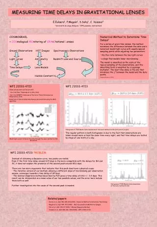
1. COSMOGRAIL = COSmological MOnitoring of GRAvItational Lenses Ground Observations HST Images Spectroscopic Observations Light curves Astrometry Redshift Lens and Source Time Delays Lens Models Hubble Constant H0 • Numerical Method to Determine Time Delays1 • For a series of given time delays, the method minimizes the difference between the data and a numerical model light curve with equally spaced sampling points while adjusting two parameters: • the flux ratio between the two light curves • a slope that models linear microlensing. • The model is smoothed on the scale of the typical sampling of the observations, and this smoothing term is weighted by a Lagrange multiplier. The best time delay is the one that minimizes the c2 between the model and the data points. • 1 Based on Burud et al. (2001) • WFI J2033-4723 • Observations were carried out with • the 1.2m Euler Telescope at La Silla, Chile • the 1.3m SMARTS telescope at the Cerro Tololo Interamerican Observatory, Chile • Reduction of data includes simultaneous deconvolution using the MCS algorithm. • Model light curves fitted on the data through the basic method for BA, BC and AC. WFI J2033-4723 Histograms of 7000 Monte Carlo simulations of the basic method for BA (left) and AC (right). The regular pattern in both histograms is due to the fact that observations are taken around more or less the same time every night, and that time delays are tested by steps of one tenth of a day. WFI J2033-4723: PROBLEM • Instead of obtaining a Gaussian curve, two peaks are visible. • Even if the first time delay around 61.9 days is the more compatible with the delays for BA and AC, it does not explain the presence of the second peak around 68.6 days. • There are two more arguments that indicate that this peak does have a physical cause: • The iterative version of our method, allowing a different slope of microlensing per observation season, converges towards a time delay of 68 days. • The minimal dispersion method described by Pelt gives a time delay of 64.6 +/- 3.4 days. This result can be interpreted as a mean value of our two possible values, and the error bars include them both as well. • Further investigation into the cause of the second peak is needed. Histogram of 7000 Monte Carlo simulations of the basic method for BC. MEASURING TIME DELAYS IN GRAVITATIONAL LENSES E.Eulaers1, P.Magain1, S.Sohy1, C. Vuissoz2 1 Université de Liège, Belgium, 2 EPFLausanne, Switzerland • Related papers • Burud et al., A&A 380, 805-810 (2001) – Numerical Method to Determine Time Delays • Magain et al, ApJ 494, 472 (1998) - MCS Deconvolution Method for Images • Pelt et al., A&A 305, 97 (1996) – Minimal Dispersion Method • Vuissoz et al., A&A 488, 481- 490 (2008) – WFI J2033-4723