The control hierarchy based on “time scale separation”
330 likes | 501 Vues
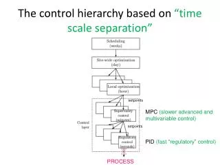
The control hierarchy based on “time scale separation”. setpoints. MPC (slower advanced and multivariable control). setpoints. PID (fast “regulatory” control ). PROCESS. Cascade control: MV for one controller (master c 1 ) is setpoint to another (slave c 2 ). . MV 1 =y s2. MV=u=P.

The control hierarchy based on “time scale separation”
E N D
Presentation Transcript
The control hierarchy based on “time scale separation” setpoints MPC (slower advanced and multivariable control) setpoints PID (fast “regulatory” control) PROCESS
Cascade control: MV for one controller (master c1) is setpoint to another (slave c2). MV1=ys2 MV=u=P Figure 15.4 Commonspecial case of “series cascade control” where y1 = gp1 y2. TexPoint fonts used in EMF. Read the TexPoint manual before you delete this box.: AAAAAAAAAAAAAAAAA
Tuning of cascade control: Example d2 d1 d2 d1 g1(s) g2(s) TexPoint fonts used in EMF. Read the TexPoint manual before you delete this box.: AAAAAAAAA
4 3.5 3 2.5 2 1.5 1 0.5 0 0 100 200 300 400 500 600 Simulation cascade control WITHOUT CASCADE y1 WITH CASCADE Setpoint change for y1 at t=0 Disturbance d2=0.1 (at input to g2, inside slave loop) at t=200 Disturbance d1=0.1 (at input to g1, outside slave loop) at t=400
PI-control: Without cascade • Integrating process with large effective delay -> control poor s=tf('s') g1 = 1/s g2 = exp(-s)/(20*s+1) y1s y1 u
PI-control: With cascade d1 d2 y1s y1 y2s y2 u
PI-control: With cascade d1 d2 y1s y1 y2s y2 u
PI-control: With cascade d1 d2 y1s y1 y2s y2 u Fast inner loop (slave loop): Takes care of disturbances inside slave loop (d2) Also have benefit of faster outer loop (master loop): Get better rejection of disturbances outside slave loop (d1) + better setpoint response (y1s)
s=tf('s') g1 = 1/s g2 = exp(-s)/(20*s+1) Kc = 0.0455 taui = 88 taud = 0 WITHOUT CASCADE d2 d1 y1s File: tunepid4_cascade0
Kc1 = 0.2000 taui1 = 20 Kc2 = 6.7000 taui2 = 12 s=tf('s') g1 = 1/s g2 = exp(-s)/(20*s+1) WITH CASCADE d1 d2 y1s File: tunepid4_cascade
4 3.5 3 2.5 2 1.5 1 0.5 0 0 100 200 300 400 500 600 Simulation cascade control WITHOUT CASCADE y1 WITH CASCADE Setpoint change for y1 at t=0 Disturbance d2=0.1 (at input to g2, inside slave loop) at t=200 Disturbance d1=0.1 (at input to g1, outside slave loop) at t=400
0.5 0.4 0.3 0.2 0.1 0 -0.1 -0.2 -0.3 -0.4 -0.5 0 100 200 300 400 500 600 Input usage (u) u WITHOUT CASCADE WITH CASCADE
Feedforward control • Model: y = g u + gd d • Measured disturbance: dm = gdm d • Controller: u = cFFdm • Ideal feedforward • y = 0 ) u = - (gd / (gdm g) d • Ideal controller: cFF = - gd/ (gdm g) • In practice: cFF(s)must be realizable • Order pole polynomial ¸ order zero polynomial • No prediction • Common simplification: cFF = k (static gain) • General:
Feedforward control (measure d1 & d2) d1: cff = -(20*s+1)/(2*s+1) d2: cff2 = -1 (not shown) d1 d2
4 3.5 3 2.5 2 1.5 1 0.5 0 0 100 200 300 400 500 600 Simulation feedforward FEEDBACK ONLY y1 FEEDFORWARD ADDED FOR d1 and d2
Multivariable control • Single-loop control (decentralized) • Decoupling • Model predictive control (MPC)
Single-loop control • Independent design • Use when small interactions (RGA=I) • Sequential design • Start with fast loop • NOTE: If close on negative RGA, system will go unstable of fast (inner) loop saturates • + Generally better performance, but • - outer loop gets slow, and • - loops depend on each other
One-wayDecoupling (improvedcontrolof y1) one-waycoupledprocess u1 y1 c1 r1-y1 D12 -g12/g11 g11g12 g21 g22 y2 c2 r2-y2 u2 DERIVATION Process: y1 = g11 u1 + g12 u2 (1) y2 = g21 u1 + g22 u2 (2) Consider u2 as disturbance for controlof y1. Think «feedforward»: Adjust u1 to make y1=0. (1) gives u1 = - (g12/g11) u2
Two-wayDecoupling: Standard implementation (Seborg) decoupledprocess = ([G-1]diag)-1 u’1 u1 y1 r1-y1 c1 -g12/g11 g11g12 g21 g22 -g21/g22 r2-y2 y2 u’2 c2 u2 … but note thatdiagonal elements ofdecoupledprocessare different from G Problem for tuning! Process: y1 = g11 u1 + g12 u2 Decoupledprocess: y1 = (g11-g21*g12/g22) u1’ + 0*u2’ Similar for y2.
Sigurd’s recommends this alternative! Two-wayDecoupling: «Inverted» implementation (Shinskey) decoupledprocess= Gdiag u’1 u1 y1 r1-y1 c1 -g12/g11 g11 g12 g21 g22 -g21/g22 r2-y2 y2 u’2 c2 u2 Advantages: (1) Decoupled process has same diagonal elements as G. Easy tuning! (2) Handles input saturation! (if u1 and u2 are actual inputs) Proof (2): y1 = g11 u1 + g12 u2, where u1 = u1’ – (g12/g11)u2. Gives : y1 = g11 u’1 + 0* u2’ Similar: y2 = 0*u1’ + g22 u2’
Model predictive control (MPC) = “online optimal control” (model) ydev=y-ys udev=u-us Discretize in time: Note: Implement only current input Δu1 Redo whole thing at each sample (move t0). Advantage MPC: Handles multivariable control, feed- forward, cascade and constraints in a unified manner
Implementation MPC project(Stig Strand, Statoil) • Initial MV/CV/DV selection • DCS preparation (controller tuning, instrumentation, MV handles, communication logics etc) • Control room operator pre-training and motivation • Product quality control Data collection (process/lab) Inferential model • Distillation: Logarithmic compositions to reduce nonlinearity, CV = - lnximpurity • MV/DV step testing dynamic models • Model judgement/singularity analysis remove models? change models? • MPC pre-tuning by simulation MPC activation – step by step and with care – challenging different constraint combinations – adjust models? • Control room operator training • MPC in normal operation, with at least 99% service factor DCS = “distributed control system” = Basic PID control layer
PDC 1021 24-HA-103 A/B 24-VA-102 24-PA-102A/B 39 21 6 17 33 34 18 1 5 48 40 35 20 LC TI 1001 1005 24LC1001.VYA 24 24 24 24 24 24 24 24 24 24 25 24 24 24 24 24 24 24 24 24 TI TI LC LC PC TI TI TI FI TI TI TI PI HC PC LC FC 1021 1018 1026 1020 1010 1015 1012 1020 1014 1013 1038 1011 1003 1009 1017 1009 1010 Depropaniser Train 100 – 24-VE-107 Flare 24 B = C2 C = C3 D = iC4 AR 1008 Kjølevann 24 FC 1008 Propane Bottoms from deetaniser 24 PD 1009 Normally 0 flow, used for start-ups to remove inerts Controlled variables (CV) = Product qualities, columndeltaP ++ 24 TC 1022 Manipulated variables (MV) =Set points to PID controllers 24 Disturbance variables (DV) = Feedforward C = C3 E = nC4 F = C5+ AR 1005 24-VE-107 LP steam Debutaniser 24-VE-108 LP condensate
Depropaniser Train100 step testing • 3 days – normal operation during night DV =Feedrate MV1 = L MV2 = Ts CV1=TOP COMPOSITION CV2=BOTTOM COMPOSITION CV3=¢p
Estimator: inferentialmodels • Analyser responsesaredelayed – temperaturemeasurementsrespond 20 min earlier • Combinetemperaturemeasurementspredictsproductqualitieswell CV1=TOP COMPOSITION Calculated by 24TI1011 (tray 39) CV2=BOTTOM COMPOSITION Calculated by 24TC1022 (t5), 24TI1018 (bottom), 24TI1012 (t17) and 24TI1011 (t39)
Depropaniser Train100 step testing – Final processmodel • Stepresponsemodels: • MV1=refluxsetpointincreaseof 1 kg/h • MV2=temperaturesetpointincreaseof 1 degree C • DV=output increaseof 1%. MV1 = L MV2 = Ts DV =Feedrate CV1=TOP COMPOSITION 3 t 20 min CV2=BOTTOM COMPOSITION CV3=¢p
Depropaniser Train100 MPC – controller activation • Starts with 1 MV and 1 CV – CV set point changes, controller tuning, model verification and corrections • Shifts to another MV/CV pair, same procedure • Interactions verified – controls 2x2 system (2 MV + 2 CV) • Expects 3 – 5 days tuning with set point changes to achieve satisfactory performance MV1 = L CV1=TOP COMPOSITION MV2 = Ts CV2=BOTTOM COMPOSITION DV =Feedrate CV3=¢p
The final test: MPC in closed-loop CV1 MV1 past predicted CV2 MV2 CV3 DV | = Present time
Conclusion MPC (Statoil) • Previous advanced control: • Cascade, feedforward, selectors, decouplers, split range control, etc. • MPC: Generally simpler • Well accepted by operators • Statoil: Use of in-house technology and expertise successful
Pole placement • Old control design method • Useful for insight, but not used in practise