String Matching Algorithms
String Matching Algorithms. Mohd. Fahim Lecturer Department of Computer Engineering Faculty of Engineering and Technology Jamia Millia Islamia New Delhi, INDIA. Searching Text. Let P be a string of size m


String Matching Algorithms
E N D
Presentation Transcript
String Matching Algorithms Mohd. Fahim LecturerDepartment of Computer Engineering Faculty of Engineering and Technology Jamia Millia Islamia New Delhi, INDIA
Let P be a string of size m • A substring P[i .. j] of P is the subsequence of P consisting of the characters with ranks between i and j • A prefix of P is a substring of the type P[0 .. i] • A suffix of P is a substring of the type P[i ..m -1] • Given strings T (text) and P (pattern), the pattern matching problem consists of finding a substring of T equal to P • Applications: • Text editors • Search engines • Biological research
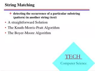
Search Text (Overview) • The task of string matching • Easy as a pie • The naive algorithm • How would you do it? • The Rabin-Karp algorithm • Ingenious use of primes and number theory • The Knuth-Morris-Pratt algorithm • Let a (finite) automaton do the job • This is optimal • The Boyer-Moore algorithm • Bad letters allow us to jump through the text • This is even better than optimal (in practice) • Literature • Cormen, Leiserson, Rivest, “Introduction to Algorithms”, chapter 36, string matching, The MIT Press, 1989, 853-885.
The task of string matching • Given • A text T of length n over finite alphabet : • A pattern P of length m over finite alphabet : • Output • All occurrences of P in T T[1] T[n] m a n a m a n a p a t i p i t i p i P[1] P[m] p a t i T[s+1..s+m] = P[1..m] m a n a m a n a p a t i p i t i p i Shift s p a t i
The Naive Algorithm Naive-String-Matcher(T,P) • n length(T) • m length(P) • for s 0 to n-m do • if P[1..m] = T[s+1 .. s+m] then • return “Pattern occurs with shift s” • fi • od Fact: • The naive string matcher needs worst case running time O((n-m+1) m) • For n = 2m this is O(n2) • The naive string matcher is not optimal, since string matching can be done in time O(m + n)
The Rabin-Karp-Algorithm • Idea: Compute • checksum for pattern P and • checksum for each sub-string of T of length m m a n a m a n a p a t i p i t i p i checksums 4 2 3 1 4 2 3 1 3 1 2 3 1 0 1 checksum 3 spurious hit valid hit p a t i
The Rabin-Karp Algorithm • Computing the checksum: • Choose prime number q • Let d = || • Example: • • Then d = 10, q = 13 • Let P = 0815 S4(0815) = (0 1000 + 8 100 + 1 10 + 5 1) mod 13 = 815 mod 13 = 9
How to Compute the Checksum: Horner’s rule • Compute • by using • Example: • • Then d = 10, q = 13 • Let P = 0815 S4(0815) = ((((010+8)10)+1)10)+5 mod 13 = ((((810)+1)10)+5 mod 13 = (3 10)+5 mod 13 = 9
How to Compute the Checksums of the Text • Start with Sm(T[1..m]) m a n a m a n a p a t i p i t i p i checksums Sm(T[1..m]) Sm(T[2..m+1])
The Rabin-Karp Algorithm Rabin-Karp-Matcher(T,P,d,q) • n length(T) • m length(P) • h dm-1 mod q • p 0 • t0 0 • for i 1 to m do • p (d p + P[i]) mod q • t0 (d t0 + T[i]) mod qod • for s 0 to n-m do • if p = ts then • if P[1..m] = T[s+1..s+m] then return “Pattern occurs with shift” s fi • if s < n-m then • ts+1 (d(ts-T[s+1]h) + T[s+m+1]) mod q fiod Checksum of the pattern P Checksum of T[1..m] Checksums match Now test for false positive Update checksum forT[s+1..s+m] usingchecksum T[s..s+m-1]
Performance of Rabin-Karp • The worst-case running time of the Rabin-Karp algorithm is O(m (n-m+1)) • Probabilistic analysis • The probability of a false positive hit for a random input is 1/q • The expected number of false positive hits is O(n/q) • The expected run time of Rabin-Karp is O(n + m (v+n/q))if v is the number of valid shifts (hits) • If we choose q ≥ m and have only a constant number of hits, then the expected run time of Rabin-Karp is O(n +m).
Boyer-Moore Heuristics • The Boyer-Moore’s pattern matching algorithm is based on two heuristics Looking-glass heuristic: Compare P with a subsequence of T moving backwards Character-jump heuristic: When a mismatch occurs at T[i] = c • If P contains c, shift P to align the last occurrence of c in P with T[i] • Else, shift P to align P[0] with T[i + 1] • Example
Last-Occurrence Function • Boyer-Moore’s algorithm preprocesses the pattern P and the alphabet S to build the last-occurrence function L mapping S to integers, where L(c) is defined as • the largest index i such that P[i]=c or • -1 if no such index exists • Example: • S = {a, b, c, d} • P=abacab • The last-occurrence function can be represented by an array indexed by the numeric codes of the characters • The last-occurrence function can be computed in time O(m + s), where m is the size of P and s is the size of S
The Boyer-Moore Algorithm Case 2: 1+l j Case 1: j 1+l AlgorithmBoyerMooreMatch(T, P, S) L lastOccurenceFunction(P, S ) i m-1 j m-1 repeat if T[i]= P[j] if j =0 return i { match at i } else i i-1 j j-1 else { character-jump } l L[T[i]] i i+ m – min(j, 1 + l) j m-1 until i >n-1 return -1 { no match }
Analysis Boyer-Moore’s algorithm runs in time O(nm + s) Example of worst case: T = aaa … a P = baaa The worst case may occur in images and DNA sequences but is unlikely in English text Boyer-Moore’s algorithm is significantly faster than the brute-force algorithm on English text
The KMP Algorithm - Motivation a b a a b x . . . . . . . a b a a b a j a b a a b a No need to repeat these comparisons Resume comparing here • Knuth-Morris-Pratt’s algorithm compares the pattern to the text in left-to-right, but shifts the pattern more intelligently than the brute-force algorithm. • When a mismatch occurs, what is the most we can shift the pattern so as to avoid redundant comparisons? • Answer: the largest prefix of P[0..j]that is a suffix of P[1..j]
KMP Failure Function • Knuth-Morris-Pratt’s algorithm preprocesses the pattern to find matches of prefixes of the pattern with the pattern itself • The failure functionF(j) is defined as the size of the largest prefix of P[0..j]that is also a suffix of P[1..j] • Knuth-Morris-Pratt’s algorithm modifies the brute-force algorithm so that if a mismatch occurs at P[j] T[i] we set j F(j-1)
The KMP Algorithm • The failure function can be represented by an array and can be computed in O(m) time • At each iteration of the while-loop, either • i increases by one, or • the shift amount i - j increases by at least one (observe that F(j-1)< j) • Hence, there are no more than 2n iterations of the while-loop • Thus, KMP’s algorithm runs in optimal time O(m + n) AlgorithmKMPMatch(T, P) F failureFunction(P) i 0 j 0 while i <n if T[i]= P[j] if j =m-1 return i -j{ match } else i i+1 j j+1 else if j >0 j F[j-1] else i i+1 return -1 { no match }
Computing the Failure Function • The failure function can be represented by an array and can be computed in O(m) time • The construction is similar to the KMP algorithm itself • At each iteration of the while-loop, either • i increases by one, or • the shift amount i - j increases by at least one (observe that F(j-1)< j) • Hence, there are no more than 2m iterations of the while-loop AlgorithmfailureFunction(P) F[0] 0 i 1 j 0 while i <m if P[i]= P[j] {we have matched j + 1 chars} F[i]j+1 i i+1 j j+1 else if j >0 then {use failure function to shift P} j F[j-1] else F[i] 0 { no match } i i+1