String Matching
String Matching. String matching problem - prefix - suffix - automata - String-matching automata - prefix function - Knuth-Morris-Pratt algorithm. Chapter 32: String Matching.

String Matching
E N D
Presentation Transcript
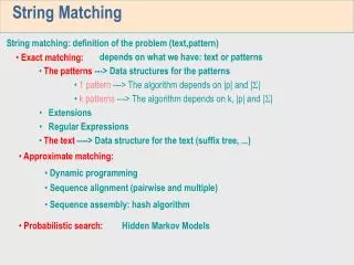
String Matching • String matching problem • - prefix • - suffix • - automata • - String-matching automata • - prefix function • - Knuth-Morris-Pratt algorithm
Chapter 32: String Matching 1. Finding all occurrences of a pattern in a text is a problem that arises frequently in text-editing programs. 2. String-matching problem text: an array T[1 .. n] containing n characters drawn from a finite alphabet . (For instance, = {1, 2} or = {a, b, …, z} pattern: an array P[1 .. m] (m n)
a c a a b c b a b c a b a a a b a s = 3 • Definition We say that pattern P occurs with shift s in text T (or, equivalently, that pattern P occurs beginning at position s + 1 in text T) if 0 s n – m and T[s + 1 .. s + m] = P[1 .. m] (i.e., if T[s + j] = P[j] for 1 j m). Valid shift s – if P occurs with shift s in T. Otherwise, s is an invalid shift. text T: pattern P: We will find all the valid shifts.
Naïve algorithm Naïve-String-Matcher(T, P) 1. n length[T] 2. m length[P] 3. fors 0 ton - m 4. doifT[s + 1 .. s + m] = P[1 .. m] 5. then print “Pattern occurs with shift” s Obviously, the time complexity of this algorithm is bounded by O(nm). In the following, we will discuss Knuth-Morris-Pratt algorithm, which needs only O(n + m) time.
0 • Knuth-Morris-Pratt algorithm - Finite automata A finite automata M is a 5-tuple (Q, q0, A, , ), where Q - a finite set of states q0 - the start state A Q – a distinguished set of accepting states - a finite input alphabet - a function from Q into Q, called the transition function of M. Example: Q = {0, 1}, q0 = 0, A = {1}, = {a, b} (0, a) = 1, (0, b) = 0, (1, a) = 0, (1, b) = 0. a input a b state 0 1 b 1 1 0 a 0 0 b
Knuth-Morris-Pratt algorithm - String-matching automata * - the set of all finite-length strings formed using characters from the alphabet - zero-length empty string |x| - the length of string x xy - the concatenation of two strings x and y, which has length |x| + |y| and consists of the characters from x followed by the characters from y prefix – a string w is a prefix of a string x, denoted w x, if x = wy for some y *. suffix - a string w is a suffix of a string x, denoted w x, if x = yw for some y *. Example:ababcca. cca abcca.
Knuth-Morris-Pratt algorithm - String-matching automata Pk - P[1 .. k] (k m), a prefix of P[1 .. m] suffix function - a mapping from * to {0, 1, …, m} such that (x) is the length of the longest prefix of P that is a suffix of x: (x) = max{k: Pkx}. Note that P0= is a suffix of every string. - Example P = ab We have () = 0 (ccaca) = 1 P = ab (ccab) = 2 P = ab
Pa a • Knuth-Morris-Pratt algorithm - String-matching automata For a pattern P[1 .. m], its string-matching automaton can be constructed as follows. 1. The state set Q is {0, 1, …, m}. The start state q0is state 0, and state m is the only accepting state. 2. The transition function is defined by the following equation, for any state q and character a: (q, a) = (Pqa) =
a a b a b a c 0 1 2 3 4 5 6 • Knuth-Morris-Pratt algorithm - Example P = ababaca a a a a 7 b b P a b a b a c a State 0 1 2 3 4 5 6 7 transition function a b c input
Knuth-Morris-Pratt algorithm - String matching by using the finite automaton Finite-Automaton-Matcher(T, , m) 1. n length[T] 2. q 0 3. fori 1 ton 4. doq (q, T[i]) 5. ifq = m 6. thenprint “pattern occurs with shift” i – m If the finite automaton is available, the algorithm needs only O(n + m) time.
b a b a a a c 0 1 2 3 4 5 6 7 • Knuth-Morris-Pratt algorithm - Example P = ababaca, T = abababacaba a a a a b b step 1: q = 0, T[1] = a. Go into the state q = 1. step 2: q = 1, T[2] = b. Go into the state q = 2. step 3: q = 2, T[3] = a. Go into the state q = 3. step 4: q = 3, T[4] = b. Go into the state q = 4. step 5: q = 4, T[5] = a. Go into the state q = 5. step 6: q = 5, T[6] = b. Go into the state q = 4. step 7: q = 4, T[7] = a. Go into the state q = 5. step 8: q = 5, T[8] = c. Go into the state q = 6. step 9: q = 6, T[9] = a. Go into the state q = 7.
Knuth-Morris-Pratt algorithm - Dynamic computation of the transition function We needn’t compute altogether, but using an auxiliary function , called a prefix function, to calculate –values “on the fly”. prefix function - a mapping from {1, …, m} to {0, 1, …, m} such that (q) = max{k: k < q, PkPq}. (x) = max{k: Pkx} comparison with suffix function:
Knuth-Morris-Pratt algorithm - Example P = ababababca i P[i] [i] P8 P6 P4 P2 P0 c a a b a b a b a b [8] = 6 [6] = 4 [4] = 2 [2] = 0 a b c a a b a b a b a b a b c a a b a b a b a b a b c a a b a b a b a b a b c a
Knuth-Morris-Pratt algorithm - function (u)(j) i) (1)(j) = (j), and ii) (u)(j) = ((u-1)(j)), for u > 1. That is, (u)(j) is just applied u times to j. Example: (2)(6) = ((6)) = (4) = 2. - How to use (u)(j)? Suppose that the automaton is in state j, having read T[1 .. k], and that T[k+1] P[j+1]. Then, apply repeatedly until it find the smallest value of u for which either 1. (u)(j) = l and T[k+1] = P[j+1], or 2. (u)(j) = 0and T[k+1] P[1]. 2(j) (j) j P: T: k
Knuth-Morris-Pratt algorithm - How to use (u)(j)? 1. (u)(j) = l and T[k+1] = P[j+1], or 2. (u)(j) = 0and T[k+1] P[1]. That is, the automaton backs up through (1)(j), (2)(j), … until either Case 1 or 2 holds for (u)(j) but not for (u-1)(j). If Case 1 holds, the automaton enters state l + 1. If Case 2 holds, it enters state 0. In either case, input pointer is advanced to position T[k+2]. In Case 1, P[1 .. j] was the longest prefix of P that is the suffix of T[1 .. k], then P[1 .. (u)(j) +1] is the longest prefix of P that is a suffix of T[1 .. k+1]. In Case 2, no prefix of P is a suffix of T[1 .. k+1].
Knuth-Morris-Pratt algorithm - Algorithm KMP-Matcher(T, P) 1. n length[T] 2. m length[P] 3. Compute-Prefix-Function(P) 4. q 0 5. fori 1 ton 6. do whileq > 0 and P[q + 1] T[i] 7. doq [q] 8. ifP[q + 1] = T[i] 9. then q q + 1 10. ifq = m 11. then print “pattern occurs with shift” i – m 12. q [q]
Knuth-Morris-Pratt algorithm - Algorithm Compute-Prefix-Function(P) 1. m length[T] 2. [1] 0 3. k 0 4. forq 2 tom 5. do whilek > 0 and P[k + 1] P[q] 6. dok [k] /*if k = 0 or P[k + 1] = P[q], 7. ifP[k + 1] = P[q] going out of the while-loop.*/ 8. then k k + 1 9. [q]k 10. return
Knuth-Morris-Pratt algorithm - Example P = ababababca, T = ababaababababca Compute prefix function [1]= 0 k = 0 q = 2, P[k + 1] = P[1] = a, P[q] = P[2] = b, P[k + 1] P[q] [q]k ([2] 0) q = 3, P[k + 1] = P[1] = a, P[q] = P[3] = a, P[k + 1] = P[q] k k + 1, [q]k ([3] 1) k = 1 q = 4, P[k + 1] = P[2] = b, P[q] = P[4] = b, P[k + 1] = P[q] k k + 1, [q]k ([4] 2)
Knuth-Morris-Pratt algorithm - Example k = 2 q = 5, P[k + 1] = P[3] = a, P[q] = P[5] = a, P[k + 1] = P[q] k k + 1, [q]k ([5] 3) k = 3 q = 6, P[k + 1] = P[4] = b, P[q] = P[6] = b, P[k + 1] = P[q] k k + 1, [q]k ([6] 4) k = 4 q = 7, P[k + 1] = P[5] = a, P[q] = P[7] = a, P[k + 1] = P[q] k k + 1, [q]k ([7] 5) k = 5 q = 8, P[k + 1] = P[6] = b, P[q] = P[8] = b, P[k + 1] = P[q] k k + 1, [q]k ([8] 6)
Knuth-Morris-Pratt algorithm - Example k = 6 q = 9, P[k + 1] = P[6] = b, P[q] = P[9] = c, P[k + 1] P[q] k [k](k [6] = 4) P[k + 1] = P[5] = a, P[q] = P[9] = c, P[k + 1] P[q] k [k](k [4] = 2) P[k + 1] = P[3] = a, P[q] = P[9] = c, P[k + 1] P[q] k [k](k [2] = 0) k = 0 q = 9, P[k + 1] = P[1] = a, P[q] = P[9] = c, P[k + 1] P[q] [q]k ([9] 0) q = 10, P[k + 1] = P[1] = a, P[q] = P[10] = a, P[k + 1] =P[q] k k + 1, [q]k ([10] 1)
Knuth-Morris-Pratt algorithm Theorem AlgorithmCompute-Prefix-Function(P) computes in O(|P|) steps. Proof. The cost of the while statement is proportional to the number of times k is decremented by the statement k [k] following do in line 6. The only way k is increased is by assigning k k + 1in line 8. Since k = 0 initially, and line 8 is executed at most (|P|) – 1 times, we conclude that the while statement on lines 5 and 6 cannot be executed more than |P| times. Thus, the total cost of executing lines 5 and 6 is O(|P|). The remainder of the algorithm is clearly O(|P|), and thus the whole algorithm takes O(|P|) time.