Partial Differential Equations
Partial Differential Equations. Definition

Partial Differential Equations
E N D
Presentation Transcript
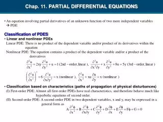
Partial Differential Equations Definition One of the classical partial differential equation of mathematical physics is the equation describing the conduction of heat in a solid body (Originated in the 18th century). And a modern one is the space vehicle reentry problem: Analysis of transfer and dissipation of heat generated by the friction with earth’s atmosphere.
For example: Consider a straight bar with uniform cross-section and homogeneous material. We wish to develop a model for heat flow through the bar. Let u(x,t) be the temperature on a cross section located at x and at time t. We shall follow some basic principles of physics: A. The amount of heat per unit time flowing through a unit of cross-sectional area is proportional to with constant of proportionality k(x) called the thermal conductivity of the material.
B. Heat flow is always from points of higher temperature to points of lower temperature. C. The amount of heat necessary to raise the temperature of an object of mass “m” by an amount u is a “c(x) m u”, where c(x) is known as the specific heat capacity of the material. Thus to study the amount of heat H(x) flowing from left to right through a surface A of a cross section during the time interval t can then be given by the formula:
Likewise, at the point x + x, we have Heat flowing from left to right across the plane during an time interval t is: If on the interval [x, x+x], during time t , additional heat sources were generated by, say, chemical reactions, heater, or electric currents, with energy density Q(x,t), then the total change in the heat E is given by the formula:
E = Heat entering A - Heat leaving B + Heat generated . And taking into simplification the principle C above, E = c(x) m u, where m = (x)V . After dividing by (x)(t), and taking the limits as x , and t 0, we get: If we assume k, c, are constants, then the eq. Becomes:
Boundary and Initial conditions Remark on boundary conditions and initial condition on u(x,t). We thus obtain the mathematical model for the heat flow in a uniform rod without internal sources (p = 0) with homogeneous boundary conditions and initial temperature distribution f(x), the follolwing Initial Boundary Value Problem:
Introducing solution of the form u(x,t) = X(x) T(t) . Substituting into the I.V.P, we obtain: The method of separation of variables
Imply that we are looking for a non-trivial solution X(x), satisfying: We shall consider 3 cases: k = 0, k > 0 and k < 0. Boundary Conditions
Case (i): k = 0. In this case we have X(x) = 0, trivial solution Case (ii): k > 0. Let k = 2, then the D.E gives X - 2 X = 0. The fundamental solution set is: { e x, e -x }. A general solution is given by: X(x) = c1 e x + c2 e -x X(0) = 0 c1 +c2 = 0, and X(L) = 0 c1 e L + c2 e -L = 0 , hence c1 (e 2L -1) = 0 c1 = 0 and so is c2 = 0 . Again we have trivial solution X(x) 0 .
Finally Case (iii) when k < 0. We again let k = - 2 , > 0. The D.E. becomes: X (x) + 2 X(x) = 0, the auxiliary equation is r2 + 2 = 0, or r = ± i . The general solution: X(x) = c1 e ix + c2 e -ix or we prefer to write: X(x) = c1 cos x + c2 sin x. Now the boundary conditions X(0) = X(L) = 0 imply: c1 = 0 and c2 sin L= 0, for this to happen, we need L = n , i.e. = n /L or k = - (n /L ) 2. We set Xn(x) = an sin (n /L)x, n = 1, 2, 3, ...
Finally for T (t) - kT(t) = 0, k = - 2 . We rewrite it as: T + 2 T = 0. Or T = - 2 T . We see the solutions are
u(x,t) = un(x,t), over all n. More precisely, This leads to the question of when it is possible to represent f(x) by the so called Fourier sine series ??
Jean Baptiste Joseph Fourier (1768 - 1830) Developed the equation for heat transmission and obtained solution under various boundary conditions (1800 - 1811). Under Napoleon he went to Egypt as a soldier and worked with G. Monge as a cultural attache for the French army.
Example Solve the following heat flow problem Write 3 sin 2x - 6 sin 5x = cn sin (n/L)x, and comparing the coefficients, we see that c2 = 3 , c5 = -6, and cn = 0 for all other n. And we have u(x,t) = u2(x,t) + u5(x,t) .
Wave Equation In the study of vibrating string such as piano wire or guitar string.
f(x) = 6 sin 2x + 9 sin 7x - sin 10x , and g(x) = 11 sin 9x - 14 sin 15x. The solution is of the form: Example:
Reminder: TA’s Review session Date: July 17 (Tuesday, for all students) Time: 10 - 11:40 am Room: 304 BH
Final Exam Date: July 19 (Thursday) Time: 10:30 - 12:30 pm Room: LC-C3 Covers: all materials I will have a review session on Wednesday
Fourier Series For a piecewise continuous function f on [-T,T], we have the Fourier series for f:
Examples Compute the Fourier series for
Convergence of Fourier Series Pointwise Convegence Theorem. If f and f are piecewise continuous on [ -T, T ], then for any x in (-T, T), we have where the an,s and bn,s are given by the previous fomulas. It converges to the average value of the left and right hand limits of f(x). Remark on x = T, or -T.
Consider Even and Odd extensions; Definition: Let f(x) be piecewise continuous on the interval [0,T]. The Fourier cosine series of f(x) on [0,T] is: and the Fourier sine series is: Fourier Sine and Cosine series
Solution Since the boundary condition forces us to consider sine waves, we shall expand f(x) into its Fourier Sine Series with T = . Thus