tompkins@ecmwft
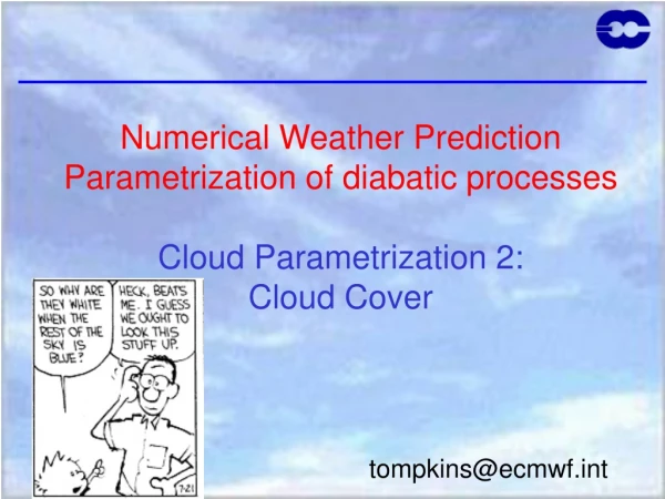
Numerical Weather Prediction Parametrization of diabatic processes Cloud Parametrization 2: Cloud Cover. tompkins@ecmwf.int. GCM Grid cell: 40-400km. Cloud Cover: The problem. Most schemes presume cloud fills GCM box in vertical Still need to represent horizontal cloud cover, a. a.

tompkins@ecmwft
E N D
Presentation Transcript
Numerical Weather Prediction Parametrization of diabatic processesCloud Parametrization 2:Cloud Cover tompkins@ecmwf.int
GCM Grid cell: 40-400km Cloud Cover: The problem Most schemes presume cloud fills GCM box in vertical Still need to represent horizontal cloud cover, a a GCM Grid
First: Some assumptions! qv = water vapour mixing ratio qc = cloud water (liquid/ice) mixing ratio qs = saturation mixing ratio = F(T,p) qt = total water (vapour+cloud) mixing ratio RH = relative humidity = qv/qs (#1) Local criterion for formation of cloud: qt > qs This assumes that no supersaturation can exist (#2) Condensation process is fast (cf. GCM timestep) qv = qs, qc= qt – qs !!Both of these assumptions are suspect in ice clouds!!
Homogeneous Distribution of water vapour and temperature: q x One Grid-cell Partial cloud cover Partial coverage of a grid-box with clouds is only possible if there is a inhomogeneous distribution of temperature and/or humidity. Note in the second case the relative humidity=1 from our assumptions
cloudy= q RH=1 RH<1 x Heterogeneous distribution of T and q Another implication of the above is that clouds must exist before the grid-mean relative humidity reaches 1.
cloudy qt RH=1 RH<1 x The interpretation does not change much if we only consider humidity variability Throughout this talk I will neglect temperature variability In fact : Analysis of observations and model data indicates humidity fluctuations are more important
qt RH=60% x 0 RH 60 80 100 Simple diagnostic schemes: RH-based schemes Take a grid cell with a certain (fixed) distribution of total water. At low mean RH, the cloud cover is zero, since even the moistest part of the grid cell is subsaturated 1 C
qt RH=80% x Simple diagnostic schemes: RH-based schemes 1 Add water vapour to the gridcell, the moistest part of the cell become saturated and cloud forms. The cloud cover is low. C 0 RH 60 80 100
qt RH=90% x Simple diagnostic schemes: RH-based schemes 1 Further increases in RH increase the cloud cover C 0 RH 60 80 100
RH=100% qt x 1 C 0 RH 60 80 100 Simple diagnostic schemes: RH-based schemes The grid cell becomes overcast when RH=100%, due to lack of supersaturation
1 C 0 RH 60 80 100 Simple Diagnostic Schemes:Relative Humidity Schemes • Many schemes, from the 1970s onwards, based cloud cover on the relative humidity (RH) • e.g. Sundqvist et al. MWR 1989: RHcrit = critical relative humidity at which cloud assumed to form (function of height, typical value is 60-80%)
Diagnostic Relative Humidity Schemes • Since these schemes form cloud when RH<100%, they implicitly assume subgrid-scale variability for total water, qt, (and/or temperature, T) exists • However, the actual PDF (the shape) for these quantities and their variance (width) are often not known • “Given a RH of X% in nature, the mean distribution of qt is such that, on average, we expect a cloud cover of Y%”
Diagnostic Relative Humidity Schemes • Advantages: • Better than homogeneous assumption, since clouds can form before grids reach saturation • Disadvantages: • Cloud cover not well coupled to other processes • In reality, different cloud types with different coverage can exist with same relative humidity. This can not be represented • Can we do better?
Diagnostic Relative Humidity Schemes • Could add further predictors • E.g: Xu and Randall (1996) sampled cloud scenes from a 2D cloud resolving model to derive an empirical relationship with two predictors: • More predictors, more degrees of freedom=flexible • But still do not know the form of the PDF. (is model valid?) • Can we do better?
Diagnostic Relative Humidity Schemes • Another example is the scheme of Slingo, operational at ECMWF until 1995. • This scheme also adds dependence on vertical velocities • use different empirical relations for different cloud types, e.g., middle level clouds: Relationships seem Ad-hoc? Can we do better?
qt x PDF(qt) qt qs Statistical Schemes • These explicitly specify the probability density function (PDF) for the total water qt (and sometimes also temperature) Cloud cover is integral under supersaturated part of PDF
LIQUID WATER TEMPERATURE conserved during changes of state Cloud mass if T variation is neglected qs S qt T Statistical Schemes • Others form variable ‘s’ that also takes temperature variability into account, which affects qs S is simply the ‘distance’ from the linearized saturation vapour pressure curve INCREASES COMPLEXITY OF IMPLEMENTATION
PDF(qt) qt C y qs x Statistical Schemes • Knowing the PDF has advantages: • More accurate calculation of radiative fluxes • Unbiased calculation of microphysical processes • However, location of clouds within gridcell unknown e.g. microphysics bias
Statistical schemes • Two tasks: Specification of the: (1) PDF shape (2) PDF moments • Shape: Unimodal? bimodal? How many parameters? • Moments: How do we set those parameters?
TASK 1: Specification of the PDF • Lack of observations to determine qt PDF • Aircraft data • limited coverage • Tethered balloon • boundary layer • Satellite • difficulties resolving in vertical • no qt observations • poor horizontal resolution • Raman Lidar • only PDF of water vapour • Cloud Resolving models have also been used • realism of microphysical parameterisation? modis image from NASA website
Aircraft Observed PDFs Wood and field JAS 2000 Aircraft observations low clouds < 2km Height Heymsfield and McFarquhar JAS 96 Aircraft IWC obs during CEPEX PDF(qt) qt
PDF Data More examples from Larson et al. JAS 01/02 Note significant error that can occur if PDF is unimodal Conclusion: PDFs are mostly approximated by uni or bi-modal distributions, describable by a few parameters
PDF( qt) qt qt Uniform: Letreut and Li (91) Triangular: Smith QJRMS (90) qt qt Gaussian: Mellor JAS (77) s4 polynomial: Lohmann et al. J. Clim (99) TASK 1: Specification of PDF Many function forms have been used symmetrical distributions:
PDF( qt) qt qt qt Lognormal: Bony & Emanuel JAS (01) Gamma: Barker et al. JAS (96) Exponential: Sommeria and Deardorff JAS (77) qt qt Beta: Tompkins JAS (02) TASK 1: Specification of PDF skewed distributions: Double Normal/Gaussian: Lewellen and Yoh JAS (93), Golaz et al. JAS 2002
Skewness Kurtosis saturation Moment 1=MEAN Moment 2=VARIANCE Moment 3=SKEWNESS Moment 4=KURTOSIS positive negative PDF(qt) cloud forms? negative positive qt e.g. HOW WIDE? TASK 2: Specification of PDF moments Need also to determine the moments of the distribution: • Variance (Symmetrical PDFs) • Skewness (Higher order PDFs) • Kurtosis (4-parameter PDFs)
(1-RHcrit)qs C G(qt) 1-C qt TASK 2: Specification of PDF moments • Some schemes fix the moments (e.g. Smith 1990) based on critical RH at which clouds assumed to form • If moments (variance, skewness) are fixed, then statistical schemes are identically equivalent to a RH formulation • e.g. uniform qt distribution = Sundqvist form where Sundqvist formulation!!!
convection turbulence microphysics dynamics Clouds in GCMsProcesses that can affect distribution moments
Example: Turbulence In presence of vertical gradient of total water, turbulent mixing can increase horizontal variability dry air moist air
Example: Turbulence In presence of vertical gradient of total water, turbulent mixing can increase horizontal variability dry air moist air while mixing in the horizontal plane naturally reduces the horizontal variability
turbulence Specification of PDF moments If a process is fast compared to a GCM timestep, an equilibrium can be assumed, e.g. Turbulence local equilibrium Source dissipation Example: Ricard and Royer, Ann Geophy, (93), Lohmann et al. J. Clim (99) • Disadvantage: • Can give good estimate in boundary layer, but above, other processes will determine variability, that evolve on slower timescales
Prognostic Statistical Scheme • I previously introduced a prognostic statistical scheme into ECHAM5 climate GCM • Prognostic equations are introduced for the variance and skewness of the total water PDF • Some of the sources and sinks are rather ad-hoc in their derivation! convective detrainment precipitation generation qs mixing
Scheme in action Minimum Maximum qsat
Turbulence breaks up cloud Scheme in action Minimum Maximum qsat
Turbulence breaks up cloud Turbulence creates cloud Scheme in action Minimum Maximum qsat
Production of variance Courtesy of Steve Klein: Change due to difference in means Transport Change due to difference in variance Also equivalent terms due to entrainment
Microphysics • Change in variance • However, the tractability depends on the PDF form for the subgrid fluctuations of q, given by G: Where P is the precipitation generation rate, e.g: Can get pretty nasty!!! Depending on form for P and G
But quickly can get untractable • E.g: Semi-Lagrangian ice sedimentation • Source of variance is far from simple, also depends on overlap assumptions • In reality of course wish also to retain the sub-flux variability too
Summary of statistical schemes • Advantages • Information concerning subgrid fluctuations of humidity and cloud water is available • It is possible to link the sources and sinks explicitly to physical processes • Use of underlying PDF means cloud variables are always self-consistent • Disadvantages • Deriving these sources and sinks rigorously is hard, especially for higher order moments needed for more complex PDFs! • If variance and skewness are used instead of cloud water and humidity, conservation of the latter is not ensured
Issues for GCMs If we assume a 2-parameter PDF for total water, and we prognose the mean and variance such that the distribution is well specified (and the cloud water and liquid can be separately derived assuming no supsaturation) what is the potential difficulty?
Which prognostic equations? Take a 2 parameter distribution & Partially cloudy conditions • Can specify distribution with • Mean • Variance • of total water • Can specify distribution with • Water vapour • Cloud water • mass mixing ratio qsat qt qsat Cloud Cloud qv ql+i Variance
qv qv+ql+i Which prognostic equations? qsat • Cloud water budget conserved • Avoids Detrainment term • Avoids Microphysics terms (almost) • Water vapour • Cloud water • mass mixing ratio qv ql+i But problems arise in Overcast conditions (…convection + microphysics) (al la Tiedtke) qsat Clear sky conditions (turbulence)
Which prognostic equations? Take a 2 parameter distribution & Partially cloudy conditions qsat • Mean • Variance • of total water • “Cleaner solution” • But conservation of liquid water compromised due to PDF • Need to parametrize those tricky microphysics terms!
Hybrid approachPartially cloudy conditions Time=i Time=i+1 * ql * ql * qv * qv q’t2 q’t2 * = used to define PDF giving cloud cover A subset of processes that are easier to handle in the PDF framework, such as turbulence, are converted into equivalent source/sink of ql and qv Variance slaved to values derived from vapour and cloud water, thus implicitly accounting for microphysical terms
Hybrid Approach: Clear sky or overcast conditions Time=i Time=i+1 ql ql * * qv qv * q’t2 * q’t2 * = used to define PDF giving cloud cover In clear sky or overcast conditions, the variance equation is fully prognostic. However in overcast conditions, the source/sink of variance from microphysics still poses a problem
qcloud If supersaturation allowed, equation for cloud-ice no longer holds qs qs qcrit qcrit PDF(qt) PDF(qt) qt qt PDF(qt) qt If assume fast adjustment, derivation is straightforward qs qcrit Much more difficult if want to integrate nucleation equation explicitly throughout cloud
Issues for GCMs What is the advantage of knowing the total water distribution (PDF)?
WRONG! Nearly all components of GCMs contain implicit/explicit assumptions concerning subgrid fluctuations e.g: RH-based cloud cover, thresholds for precipitation evaporation, convective triggering, plane parallel bias corrections for radiative transfer… etc. You might be tempted to say… Hurrah! We now have cloud variability in our models, where before there was none!
‘N’ Metrics e.g. Z500 scores, TOA radiation fluxes ‘M’ tuning parameters Variability in Clouds Is this desirable to have so many independent tunable parameters? With large M, task of reducing error in N metrics Becomes easier, but not necessarily for the right reasons Solution: Increase N, or reduce M
Statistical Cloud Scheme Advantage of Statistical Scheme Microphysics Convection Scheme Can use information in Other schemes Thus ‘complexity’ is not synonymous with ‘M’: the tunable parameter space Radiation
Use variance to calculate Effective thickness Approximation Effective Liquid = K x Liquid Cahalan et al 1994 G(qt) ETA adjustment Total Water qsat Use Moments to find best-fit Gamma Distribution PDF and apply Gamma weighted TSA Barker (1996) Gamma Function G(qt) Total Water qsat Thick Cloud etc. G(qt) Split PDF and perform N radiation calculations Total Water qsat Use in other Schemes (II) IPA Biases Knowing the PDF allows the IPA bias to be tacked

