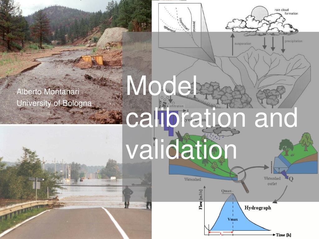
1. Model calibration and validation Alberto Montanari University of Bologna

2. Why hydrological models need to be calibrated? • Parameters: A parameter is a constant or variable term in a function that determines the specific form of the function but not its general nature, as a in f (x) = ax, where a determines only the slope of the line described by f(x). Parameters might be present in fully physically-based equations (physical properties can be considered as parameters) but usually the term parameter is reserved for quantities that are not physically measurable and compensate for approximations in physical equations.

3. Why hydrological models need to be calibrated? Hydrological models only provide an approximation of the underlying actual processes. Therefore they exhibit a certain degree of conceptualisation and parameters are not physically measurable. Calibration allows us to “adapt” model equations to specific case studies and applications. Calibration is usually performed by “adapting” the model output to observed data. However, it is possible to calibrate models also basing on personal experience and perception of the processes.

4. Calibration procedures • Manual calibration: trial and error, perceptional • Automatic calibration • - Optimisation algorithms • - Evolutionary algorithms • - Genetic algorithms (Genoud in R) • Need to define an objective function to automatically quantify the goodness of the fit.

5. Objective functions • Least squares • Nash-Sutcliffe efficiency • Correlation coefficient

6. Objective functions • These are quadratic measures • Mean relative error

7. Calibration problems • Overfitting • Equifinality • Correlation among parameters • Need to use all the available information • Multiobjective calibration • Non dominated solutions and Pareto fronteer

8. Model validation • Calibration assures the best fit of the observed data. It does not give any indication about model performances in real world applications. • Need to check how the model works with out-of-sample applications. • Split sample calibration and validation. • Jack-knife validation

9. Visual comparison between observed and simulated data • Graph of observed vs simulated hydrographs

10. Visual comparison between observed and simulated data • Scatterplot of observed vs simulated hydrographs

11. Visual comparison between observed and simulated data • Comparison of observed vs simulated flow duration curves • Flow duration curve: a graph showing observed river flows in the Y ax versus the average time span in a year during which each river flow observation was equalled or exceeded. Usually estimated by using daily data

12. What is a good model? • Difficult to say but: • - Nash efficiency in the range 0.6-0.9 • - Correlation coefficient in the range 0.8-0.99 • - Mean relative error in the range 15% – 40% • - Mean relative error in the simulation of peak flows in the range 10% - 25% • - No evidence of significant model structural inadequacy for different river flow regimes.