Advanced Techniques for Solving Rendering and Potential Equations in Computer Graphics
300 likes | 433 Vues
This document outlines various strategies for addressing rendering and potential equations, focusing on techniques like recursive ray tracing and approximations for solving the rendering equation. It explores local and global illumination models, the impact of light source visibility, and provides examples of iterative, expansion, and inversion methods for achieving approximate solutions. The text also discusses the coupling of variables in rendering equations, revealing computational alternatives for more efficient rendering while maintaining realism through light simulation.

Advanced Techniques for Solving Rendering and Potential Equations in Computer Graphics
E N D
Presentation Transcript
Strategies to solve the rendering or potential equations László Szirmay-Kalos
Coupling in the rendering equation L(x,w)=Le(x,w)+L(h(x,-w),w)fr (’,x,) cos ’dw’ L(h(x,-w),w) h(x,-w) L(x,w) ’ ’ w x fr (’,x,)
Compromises in the solution • Ignore all types of coupling: • local illumination models • Follow just very specific types of coupling that have finite number: • recursive ray-tracing • Resolve the coupling: • global illumination models
Example: x = 0.1 x + 1.8Solution by ignoring the coupling • Ignoring the coupling: • right side’s x: x = 0.1 x + 1.8 1.8 • Approximate solution: • x = 0.1·1.8 + 1.9 = 1.98
Local illumination models • The radiance of in the right side: • is replaced by an approximation of the emission function: abstract lightsources • Single reflection of the light from the abstract lightsources are computed L(x,w)=Le(x,w)+Llightsource fr (’,x,) cos ’dw’ Le(x,w)
Lightsource models • Ambient lightsource: La constant • ambient refl. model: Lref = La ka • Sky-light model: Lref = La a(x, view dir) • Directional lightsource • radiates into a single direction, the intensity is independent of the position • Positional lightsource • radiates from a single position, the intensity decreases with the square distance
Local illumination algorithms pixel • Visibility computation from the eye • Lightsource visibility from the visible point • Calculation of the reflection of the light from the lightsources
Result of local illumination models Without lightsource visibility computation With lightsource visibility computation
Recursive ray-tracing • The radiance of in the right side is replaced by an approximation of the emission function and by the radiance from ideal refraction and refraction directions • Single incoherent reflection and multiple coherent reflections of the light from the abstract lightsources are computed L(x,w)=Le(x,w)+ + Llightsource fr (’,x,) cos ’dw’ + krLin (x, wr) + ktLin(x, wt)
refracted ray reflected ray shadow rays Llightsource Recursive ray-tracing
Comparison of the solution alternatives of L = Le +tL Local illumination with shadows 0.1 sec … sec Recursive ray tracing secs… mins Global illumination mins … hours
Global illumination solution • Inversion • Expansion • Iteration (1- )L = Le L = (1- ) -1Le L = Le+L = Le+Le+2L= Le+Le+2 Le +3L = nLe Ln = Le+ Ln-1
Example: x = 0.1 x + 1.8Solution by inversion • Grouping the unknown terms: • 0.9 x = 1.8 • Inversion: • x = 0.9 -1 1.8 = 2 • Luck: multiplication by a scalar is invertible
Inversion (1- )L = Le L = (1- ) -1Le • is infinite dimensional • it requires finite approx. of and the radiance L : • finite element techniques
Example: x = 0.1 x + 1.8Solution by expansion • xi=1.8+0.1 1.8 +0.121.8 + …+ 0.1i+1x • i: 1 2 3 4 • xi sequence: 1.8 1.98 1.998 1.9998
Expansion L=Le+L=Le+Le+2L=nLe ifnL 0 • should be a contraction • Rendering equation: • radiance: • measured power: • Potential equation: • potential: • measured power: L = nLe F= ML = M nLe W = ’ n We F= M’W = M’ nWe
Error of truncating the Neumann series ML = M nLe DM nLe error= |n=D+1M nLe |=|M D+1( n=0 nLe )| qD+1F || L|| q||L||, q is the contraction
Terms of the expansion of the rendering equation: 1-bounce M(Le) = P R(p,w1) Le(y,-w1) dw1dp Le y L(x,w) ’1 w1 w p x R(p,w1) = 1/Spfr (w1,x,) cos’1
Terms of the expansion of the rendering equation: 2-bounce M(2Le)=P R(p,w1,w2)Le(z,-w2) dw1dw2dp Gathering walks y w2 L(x,w) ’1 z ’2 w1 w p x Le R(p,w1,w2) = 1/Spfr (w1,x,)cos’1 fr (w2,y,1)cos’2
Terms of the expansion of the potential equation: 1-bounce M’(’We)= S Le(x,w)cos{ We(y,w1) fr(w,y,1)cos1dw1 }dwdx = S Le(x,w)cosfr(w,y,eye)g(y)dwdx=S Le(x,w)R(x,w)dwdx x w Le (x,w) p 1 weye y R(x,w) = cos fr (w,y,eye) g(y)
Terms of the expansion of the potential equation: 2-bounce F=M’(’2We)=S R(x,w,w1) Le(x,w) dw1dwdx Shooting walks y w1 p x 2 1 w weye z Le (x,w) R(x,w,w1) = cos fr (w,y,1)cos1 fr (w1,z,eye) c(p)
Expansion is a series of high dimensional integrals R(w1,...,wn,x) = w1 w2 …wn wi= fr cos ’ pixel w 1 e w L 2 F=n...R(w1,...,wn,x)Le(w1,...,wn,x)dw1,...,dwndx 1/M iM nDR(w1(i),...,wn(i),x(i) )Le(w1(i),...,wn(i),x(i)) • It requires just discrete samples from Le and R • No finite elements are needed
Example: x = 0.1 x + 1.8Solution by iteration • Iteration scheme: • xn = 0.1 xn-1 + 1.8, • n: 1 2 3 4 • xnsequence:0 1.8 1.98 1.998 1.9998
Iteration Ln = Le+ Ln-1 • Requirements of convergence • Convergent: Ln = Le+ Ln-1 Ln -1 = Le+ Ln-2 |Ln-Ln-1| = |(Ln-1-Ln-2)| = |n-1(L1-L0)| lim |n-1(L1-L0)| = 0
If is a contraction • || L || q||L||, • q < 1contraction ratio = albedo • ||n-1(L1-L0) || q n-1||L1-L0|| • converges with the speed of the geometric series e.g.: • ||L||1=, q is the average albedo
Error analysis of the iteration • Assume that is only approximated by * • L1 = Le+* L= L+L • L2 = Le+* L1 = L+L+* L • … • Ln = Le+* Ln-1 = L+L+*L+*2 L+... • ||L-L||||L||+||*L||+…=||L||(1+q+q2+…) ||L-L|| || L- * L || / (1-q)
Analitically solvable cases • Normal approach: scene radiance solution • Inverse approach: radiance scene • Good for testing global illumination algorithms • constant radiance • constant reflected radiance
Constant radiance L (x,w) = L* L*= Le (x,w)+tL* = Le (x,w)+L*t1 = Le (x,w)+L* a(x,w) • a(x,w) = 1 - Le (x,w)/ L* • arbitrary geometry in a closed environment
Constant reflected radiance L (x,w) = Le (x,w)+Lr* Le +Lr* = Le +t(Le +Lr* ) = Le +t(Le +Lr* )= Le +tLe +Lr*t1 = Le +tLe +Lr*a(x,w) • a(x,w) = 1 - tLe(x,w)/ Lr* • special case: constant albedo?
R y x’ y x |x-y| Spherical geometry with diffuse emission: constant reflected radiance tLe= Le(h(x,-w’)) fr cosx’ dw’ = S fr cosx’ cosyLe(y)/|x-y|2 dy cosx’=cosy=|x-y|/2R tLe=fr S Le(y) dy 4R2 =albedo average(Le)