Demand Analysis
Demand Analysis. Some Questions. What is behind a consumer’s demand curve? How do consumers choose from among various consumer “goods”? What determines the value of a consumer good?. What is Consumer Theory?. Study of how people use their limited means to make purposeful choices.

Demand Analysis
E N D
Presentation Transcript
Some Questions • What is behind a consumer’s demand curve? • How do consumers choose from among various consumer “goods”? • What determines the value of a consumer good?
What is Consumer Theory? • Study of how people use their limited means to make purposeful choices. • Assumes that consumers understand their choices (possibilities) and the prices (opportunity costs) associated with each choice. • Assumes that consumers consider the alternatives and choose the one they like best.
Consumer Theory - Why? • Two important reasons: • to understand the foundations of market demand (bake the demand curve from scratch) • to address several interesting consumer theory issues that are best understood using this model rather than the aggregate demand model
Two Components of Consumer Demand • Opportunities: • What can the consumer afford? • What are the consumption possibilities? • Summarized by the budget constraint • Preferences: • What does the consumer like? • How much does a consumer like a good? • Summarized by the utility function
Utility • The value a consumer places on a unit of a good or service depends on the pleasure or satisfaction he or she expects to derive form having or consuming it at the point of making a consumption (consumer) choice. • In economics the satisfaction or pleasure consumers derive from the consumption of consumer goods is called “utility”. • Consumers, however, cannot have every thing they wish to have. Consumers’ choices are constrained by their incomes. • Within the limits of their incomes, consumers make their consumption choices by evaluating and comparing consumer goods with regard to their “utilities.”
Our basic assumptions about a “rational” consumer: • Consumers are utility maximizers • Consumers prefer more of a good (thing) to less of it. • Facing choices X and Y, a consumer would either prefer X to Y or Y to X, or would be indifferent between them. • Transitivity: If a consumer prefers X to Y and Y to Z, we conclude he/she prefers X to Z • Diminishing marginal utility: As more and more of good is consumed by a consumer, ceteris paribus, beyond a certain point the utility of each additional unit starts to fall.
How to Measure Utility Measuring utility in “utils” (Cardinal): • Jack derives 10 utils from having one slice of pizza but only 5 utils from having a burger. • In many introductory microeconomics textbooks this approach to measuring utility is still considered effective for teaching purposes. Measuring utility by comparison (Ordinal): • Jill prefers a burger to a slice of pizza and a slice of pizza to a hotdog. Often consumers are able to be more precise in expressing their preferences. For example, we could say: • Jill is willing to trade a burger for four hotdogs but she will give up only two hotdogs for a slice of pizza. • We can infer that to Jill, a burger has twice as much utility as a slice of pizza, and a slice of pizza has twice as much utility as a hotdog.
Utility and Money • Because we use money (rather than hotdogs!) in just about all of our trade transactions, we might as well use it as our comparative measure of utility. (Note: This way of measuring utility is not much different from measuring utility in utils) • Jill could say: I am willing to pay $4 for a burger, $2 for a slice of pizza and $1 for a hotdog. Note: Even though Jill obviously values a burger more (four times as much) than a hot dog, she may still choose to buy a hotdog, even if she has enough money to buy a burger, or a slice of pizza, for that matter. (We will see why and how shortly.)
Total Utility versus Marginal Utility • Marginal utility is the utility a consumer derives from the last unit of a consumer good she or he consumes (during a given consumption period), ceteris paribus. • Total utility is the total utility a consumer derives from the consumption of all of the units of a good or a combination of goods over a given consumption period, ceteris paribus. Total utility = Sum of marginal utilities
The Law of Diminishing Marginal Utility • Over a given consumption period, the more of a good a consumer has, or has consumed, the less marginal utility an additional unit contributes to his or her overall satisfaction (total utility). • Alternatively, we could say: over a given consumption period, as more and more of a good is consumed by a consumer, beyond a certain point, the marginal utility of additional units begins to fall.
How much ice cream does Jill buy in a month? Some facts of life: • Limited income • Opportunity cost of making a choice: Buying ice cream leaves Jill less money to buy other things: each dollar spent on ice cream could be spent on hamburger. • In fact, consumers compare the (expected) utility derived from one additional dollar spent on one good to the utility derived from one additional dollar spent on another good.
What is a Budget Constraint? • A budget constraint shows the consumer’s purchase opportunities as every combination of two goods that can be bought at given prices using a given amount of income. • The budget constraint measures the combinations of purchases that a person can afford to make with a given amount of monetary income.
Units of A Price $1.50 Units of B Price $1.00 12 10 8 6 4 2 0 Total Expenditures Quantity of A 2 4 6 8 10 12 Quantity of B THE BUDGET LINE: What is Attainable 8 0 $12 6 3 12 4 6 12 2 9 12 0 12 12
Units of A Price $1.50 Units of B Price $1.00 12 10 8 6 4 2 0 Total Expenditures 2 4 6 8 10 12 THE BUDGET LINE: What is Attainable 8 0 $12 6 3 12 4 6 12 2 9 12 0 12 12 Quantity of A Quantity of B
Units of A Price $1.50 Units of B Price $1.00 12 10 8 6 4 2 0 Total Expenditures 2 4 6 8 10 12 THE BUDGET LINE: What is Attainable 8 0 $12 6 3 12 4 6 12 2 9 12 0 12 12 Quantity of A Quantity of B
Units of A Price $1.50 Units of B Price $1.00 12 10 8 6 4 2 0 Total Expenditures 2 4 6 8 10 12 THE BUDGET LINE: What is Attainable 8 0 $12 6 3 12 4 6 12 2 9 12 0 12 12 Quantity of A Quantity of B
Units of A Price $1.50 Units of B Price $1.00 12 10 8 6 4 2 0 Total Expenditures 2 4 6 8 10 12 THE BUDGET LINE: What is Attainable 8 0 $12 6 3 12 4 6 12 2 9 12 0 12 12 Quantity of A Quantity of B
Units of A Price $1.50 Units of B Price $1.00 12 10 8 6 4 2 0 Total Expenditures 2 4 6 8 10 12 THE BUDGET LINE: What is Attainable 8 0 $12 6 3 12 4 6 12 2 9 12 0 12 12 (Unattainable) Quantity of A (Attainable) Quantity of B
Units of A Price $1.50 Units of B Price $1.00 12 10 8 6 4 2 0 Total Expenditures An Increase in income makes the purchase of more of either or both items possible 2 4 6 8 10 12 THE BUDGET LINE: What is Attainable 8 0 $12 6 3 12 4 6 12 2 9 12 0 12 12 (Unattainable) Quantity of A (Attainable) Quantity of B
Units of A Price $1.50 Units of B Price $1.00 12 10 8 6 4 2 0 Total Expenditures Price changes cause a change in the quantity demanded of the items 2 4 6 8 10 12 THE BUDGET LINE: What is Attainable 8 0 $12 6 3 12 4 6 12 2 9 12 0 12 12 (Unattainable) Quantity of A (Attainable) Quantity of B
Units of A Price $1.50 Units of B Price $1.00 12 10 8 6 4 2 0 Total Expenditures Combi- nation Units of A Units of B 2 4 6 8 10 12 INDIFFERENCE CURVES What is Preferred j 8 0 $12 6 3 12 4 6 12 2 9 12 0 12 12 Quantity of A An Indifference Schedule j 12 2 Quantity of B
Units of A Price $1.50 Units of B Price $1.00 12 10 8 6 4 2 0 Total Expenditures 2 4 6 8 10 12 INDIFFERENCE CURVES What is Preferred j 8 0 $12 6 3 12 4 6 12 2 9 12 0 12 12 k Quantity of A An Indifference Schedule Combi- nation Units of A Units of B j 12 2 k 6 4 Quantity of B
Units of A Price $1.50 Units of B Price $1.00 12 10 8 6 4 2 0 Total Expenditures 2 4 6 8 10 12 INDIFFERENCE CURVES What is Preferred j 8 0 $12 6 3 12 4 6 12 2 9 12 0 12 12 k Quantity of A l An Indifference Schedule Combi- nation Units of A Units of B j 12 2 k 6 4 l 4 6 Quantity of B
Units of A Price $1.50 Units of B Price $1.00 12 10 8 6 4 2 0 Total Expenditures 2 4 6 8 10 12 INDIFFERENCE CURVES What is Preferred j 8 0 $12 6 3 12 4 6 12 2 9 12 0 12 12 k Quantity of A l An Indifference Schedule m Combi- nation Units of A Units of B j 12 2 k 6 4 l 4 6 m 3 8 Quantity of B
Units of A Price $1.50 Units of B Price $1.00 12 10 8 6 4 2 0 Total Expenditures 2 4 6 8 10 12 INDIFFERENCE CURVES What is Preferred j 8 0 $12 6 3 12 4 6 12 2 9 12 0 12 12 k Quantity of A l An Indifference Schedule m Combi- nation Units of A Units of B I j 12 2 k 6 4 l 4 6 m 3 8 Quantity of B
Units of A Price $1.50 Units of B Price $1.00 12 10 8 6 4 2 0 Total Expenditures 2 4 6 8 10 12 INDIFFERENCE CURVES What is Preferred j The slope represents the marginal rate of substi- tution, (MRS) 8 0 $12 6 3 12 4 6 12 2 9 12 0 12 12 k Quantity of A l An Indifference Schedule m Combi- nation Units of A Units of B I2 I1 j 12 2 k 6 4 l 4 6 m 3 8 Quantity of B
Units of A Price $1.50 Units of B Price $1.00 12 10 8 6 4 2 0 Total Expenditures If the consumer had greater income, more of either or both products could be purchased 2 4 6 8 10 12 INDIFFERENCE CURVES What is Preferred 8 0 $12 6 3 12 4 6 12 2 9 12 0 12 12 Quantity of A An Indifference Schedule Combi- nation Units of A Units of B I1 j 12 2 k 6 4 l 4 6 m 3 8 Quantity of B
Units of A Price $1.50 Units of B Price $1.00 12 10 8 6 4 2 0 Total Expenditures A higher combination of choices will be preferred 2 4 6 8 10 12 INDIFFERENCE CURVES What is Preferred 8 0 $12 6 3 12 4 6 12 2 9 12 0 12 12 Quantity of A An Indifference Schedule I4 I3 Combi- nation Units of A Units of B I2 I1 j 12 2 k 6 4 l 4 6 m 3 8 Quantity of B
Units of A Price $1.50 Units of B Price $1.00 12 10 8 6 4 2 0 Total Expenditures A family of all such expressions of indifference can be developed for every level of income 2 4 6 8 10 12 INDIFFERENCE CURVES What is Preferred 8 0 $12 6 3 12 4 6 12 2 9 12 0 12 12 An Indifference Map Quantity of A An Indifference Schedule I4 I3 Combi- nation Units of A Units of B I2 I1 j 12 2 k 6 4 l 4 6 m 3 8 Quantity of B
Units of A Price $1.50 Units of B Price $1.00 12 10 8 6 4 2 0 Total Expenditures 2 4 6 8 10 12 EQUILIBRIUM AT TANGENCY 8 0 $12 6 3 12 4 6 12 2 9 12 0 12 12 (Unattainable) Quantity of A An Indifference Schedule I4 I3 Combi- nation Units of A Units of B I2 (Attainable) I1 j 12 2 k 6 4 l 4 6 m 3 8 Quantity of B
12 10 8 6 4 2 0 2 4 6 8 10 12 EQUILIBRIUM AT TANGENCY Equilibrium occurs when the consumer selects the combination which reaches the highest attainable indifference curve. (Unattainable) Quantity of A I4 I3 I2 (Attainable) I1 Quantity of B
12 10 8 6 4 2 0 2 4 6 8 10 12 EQUILIBRIUM AT TANGENCY What happens if the price of B increases to$1.50? The budget line rotates reflecting the reduction in the quantity of B units which is attainable. QuantityB PriceB $1.00 6 Quantity of A I3 Quantity of B
12 10 8 6 4 2 0 2 4 6 8 10 12 EQUILIBRIUM AT TANGENCY What happens if the price of B increases to$1.50? The budget line rotates reflecting the reduction in the quantity of B units which is attainable. QuantityB PriceB $1.00 1.50 6 3 Quantity of A I3 By recording the various quantities demanded at the various prices yields the Demand schedule I2 Quantity of B
12 10 8 6 4 2 0 2 4 6 8 10 12 EQUILIBRIUM AT TANGENCY What happens if the price of B increases to$1.50? The budget line rotates reflecting the reduction in the quantity of B units which is attainable. QuantityB PriceB $1.00 1.50 6 3 Quantity of A I3 By recording the various quantities demanded at the various prices yields the Demand schedule I2 Quantity of B
DERIVING THE DEMAND CURVE What happens if the price of B increases to$1.50? Plotting the Points yields the Demand Curve for Product B Price of B $1.50 1.00 0 QuantityB PriceB $1.00 1.50 6 3 DB By recording the various quantities demanded at the various prices yields the demand schedule. 2 4 6 8 10 12 Quantity of B