Download
1 / 21
210 likes | 323 Vues
Advancing Numerical Weather Prediction of Great Salt Lake-Effect Precipitation. John D McMillen. Questions and Hypotheses.

E N D
Advancing Numerical Weather Prediction of Great Salt Lake-Effect Precipitation John D McMillen
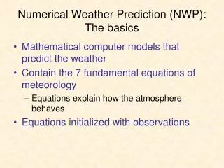
Questions and Hypotheses • How and why does the choice of microphysical parameterization in numerical weather prediction models affect quantitative GSLE precipitation forecasts at convection-permitting (~1 km) grid spacing comparable to those likely to be available to forecasters during the next decade? • We hypothesize quantitative GSLE precipitation forecasts will be affected by the choice of microphysics parameterizations at convection-permitting grid spacing for three reasons. • Microphysical parameterizations were designed to simulate specific phenomena • The tendency equations within each different microphysical parameterization are frequently unique • Even when hydrometeor tendency equations are theoretically the same, the way they are used may yield a different result
Research Methods - MP Study • GSLE simulation sensitivity to microphysics choice • Case study of 27 Oct 2010 event • Control Run WRF ARW 3.4 • 1.33 km inner domain (3rd single nested domain) • NAM LBC, Cold start • 35 vertical levels • 8 sec integration time step • Thompson microphysics parameterization • Kain-Fritsch convective parameterization on outer domains, none on inner domain • YSU PBL parameterization • NOAH LSM parameterization • RRTM (SW) and RRTMG (LW) radiation parameterizations • Simple second order diffusion • 2D Smagorinsky eddy coefficient
D1 12 km D2 4 km D3 1.3 km
GSLE Precip Subdomain B MP Subdomain A
Total Precipitation 0230-1700 UTC 27 October 2010 NEXRAD Thompson • Liquid equivalent precip derived from NEXRAD with Z = 75S2 relationship • NEXRAD plot compares well with surface observations over the valley, but underestimates liquid equivalent precipover the high Wasatch
Research Methods - MP Study • All simulations generated similar synoptic fields • Moisture was similar • Over-lake convergence bands were generated in every simulation • This consistency implies that GSLE precipitation distribution and amount differences between simulations are caused by the choice of MP scheme
Total Precipitation 0230-1700 UTC 27 October 2010 Thompson Goddard WDM6 Morrison
Precipitation Statistics 0230-1700 UTC, 27 October 2010 Statistics calculated over GSLE Precip Subdomain
Hydrometer Mass Profiles Values averaged over MP Subdomain from 0230-1700 UTC
Hydrometer Mass Profiles Values averaged over MP Subdomain from 0230-1700 UTC
Hydrometer Mass Profiles Values averaged over MP Subdomain from 0230-1700 UTC
Hydrometeor Tendency Equations • We extracted the source and sink terms of the snow hydrometeor tendency equations • THOM • qsten(k) = qsten(k) + (prs_iau(k) + prs_sde(k) + prs_sci(k) + prs_scw(k) + prs_rcs(k) + prs_ide(k) - prs_ihm(k) - prr_sml(k))*orho • WDM6 • qrs(i,k,2) = max(qrs(i,k,2) + (psdep(i,k) + psaut(i,k) + paacw(i,k) - pgaut(i,k) + piacr(i,k)*delta3 + praci(i,k)*delta3 + psaci(i,k) - pgacs(i,k) - pracs(i,k)*(1. - delta2) + psacr(i,k)*delta2)*dtcld , 0.)
Hydrometeor Tendency Equations • We extracted the source and sink terms of the graupel hydrometeor tendency equation • THOM • qgten(k) = qgten(k) + (prg_scw(k) + prg_rfz(k) + prg_gde(k) + prg_rcg(k) + prg_gcw(k) + prg_rci(k) + prg_rcs(k) - prg_ihm(k) - prr_gml(k))*orho • WDM6 • qrs(i,k,3) = max(qrs(i,k,3) + (pgdep(i,k) + pgaut(i,k) + piacr(i,k)*(1.-delta3) + praci(i,k)*(1. - delta3) + psacr(i,k)*(1.-delta2) + pracs(i,k)*(1.-delta2) + pgaci(i,k) + paacw(i,k) + pgacr(i,k) + pgacs(i,k))*dtcld, 0.)
SnowTendency Profiles • Values averaged over MP Subdomain from 0230-1700 UTC • Solid lines are the sum of all terms
GraupelTendency Profiles • Values averaged over MP Subdomain from 0230-1700 UTC • Solid lines are the sum of all terms
Total Graupel0230-1700 UTC 27 October 2010 WDM6 Thompson
Total Precipitation 0230-1700 UTC 27 October 2010 Thompson Goddard WDM6 Morrison
Precipitation Pattern • All schemes displace the band of maximum precipitation to the southwest compared to observations • Thompson is closest to observations, but still displaced • The precipitation location is driven by the convergence axis Thompson WDM6 Divergence averaged through the lowest 2 sigma levels ( green < 0 s-1 ; yellow < -110 s-1 ; interval -30 s-1) and lowest sigma level winds (full barb = 5 m s-1) 0230 UTC 27 Oct 2010
Predecessor Precipitation • Precipitation produced by a baroclinic trough before 0230 UTC differs between schemes WDM6 WDM6 B A A B Precipitation difference 1800 UTC 26 Oct through 0230 UTC 27 Oct WDM6 – Thompson 8 km horizontal average circulation and potential temp over potential temp difference WDM6 – Thompson
Predecessor Precipitation • All Schemes produce poor precipitation from the baroclinic trough compared to NEXRAD • Poor synoptic precipitation distribution affects GSLE precipitation distribution NEXRAD Thompson