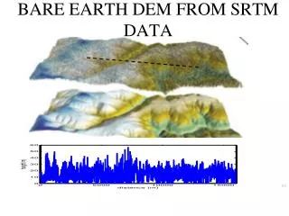
BARE EARTH DEM FROM SRTM DATA
BARE EARTH DEM FROM SRTM DATA. CG. Objective of the project. Improve Digital Elevation Models (DEMs) from SRTM mission for hydrodynamic modeling and other applications. Obtain spatial and temporal structure of vegetation biomass.

BARE EARTH DEM FROM SRTM DATA
E N D
Presentation Transcript
Objective of the project • Improve Digital Elevation Models (DEMs) from SRTM mission for hydrodynamic modeling and other applications. • Obtain spatial and temporal structure of vegetation biomass. • Obtain a high resolution bare-earth DEM (90m) for areas where the elevation data is not available.
Sensor dependence: Vegetation appears as uniformly distributed noise at some scales at SRTM 30 m NED data @30 m SRTM Data @ 30 m
SRTM VEGETATION RESPONSE • A Fundamental law of science applies to the SRTM data • “ One scientist’s noise is another scientist’s signal”
Fourier Analysis • Vege. Topo. = bare earth Topo.+ veg. ht Unknown, but at large scale bare-earth topo. Amplitude is approximately equals to the amplitude of the SRTM signal. Phase is unknown and will be resolved iteratively Unknown, but we have shown that phase of the veg. height can be obtained using SRTM signal. Amplitude can will be resolved iteratively Known from SRTM Signal We have two equations in the Fourier domain and two unknowns- can be resolved. Can be extended to the 2D
Spatial domain frequency domain Real part Imaginary part
Fourier based approach • Linearity of the Fourier transform is used. • If: x1[n] + x2[n] = x3[n], • then: ReX1[f] + ReX2[f] = ReX3[f] and ImX1[f] + ImX2[f] = ImX3[f].
Additively in Spectral Domain: proposed model Fourier Amplitude Fourier Phase
Fourier Power spectrum : vegetation topography, bare-earth, and vegetation height- SF Eel LiDAR data
Study area 3: Tenderfoot Creek Vertical profiles Vegetation fractional cover ~ 90
A Simple approach: • Low frequency content of the vegetation topography is coming from bare-earth topography • High frequency content of the vegetation topography is coming from the vegetation height. • Two regions are separated by a scale break at frequency fc
Approach…. low frequency content~ bare-earth topo. High frequency content~ vegetation height
Model parameters-Amplitudes of the bare-earth and vegetation topography: LiDAR data at low frequencies
Model parameters-phase of the bare-earth and vegetation topography: at low frequencies
Canopy topography phase VS Canopy height phase CANOPY HEIGHT PHASE CAN BE OBTAINED! AMPLITUDE CAN BE RESOLVED ITERATIVELY
Back to the model equations.. For bare-earth = and = The low frequency content is obtained using model eqn. The high frequency information of the bare-earth is obtained by Fourier interpolations
model…. For vegetation height = and = High frequency contact is obtained from the model eqn. The low frequency information of the bare-earth is obtained by Fourier interpolations
Results: A comparison of Model topo. and LiDAR bare-earth: It preserves the second order moments
Conclusions: • Vegetation topography leaves a clear statistical signature about the vegetation height and the bare-earth ( can be extracted using minimally used ancillary data.) • A clear signature of the vegetation height data – two power law scaling regimes (i.e., low frequency and high frequency) with a scaling break at a intermediate characteristic frequency. • The characteristic frequency depends on the vegetation density and the grid resolution • vegetation mainly distort bare-earth power law scaling regime at the high frequency range • If the objective is the canopy model (hydrodynamic model) model resolution should be selected from low frequency (high frequency) range.
Can we improve our solution! • Fourier approach can not localized spatially! • Solution obtained from iterative optimization may not be always realistic. • Can we integrate remotely sensed ground truth data to obtain realistic solutions • We want to zoom down to vegetation patch scales and implement scale dependant interpolating approach to remove the vegetation effect/ obtain the vegetation height while preserving observed statistical properties of the bare earth
SCALE 1 SACLE 2 SCALE 3 SCALE 4 SCALE 5 Chandana Gangodagamage
FUSION OF DIFFERENT SENSOR DATA ASTER and SRTM
TfTgTvAfAgAv eq1= 'Af/(1+(tan(Tf))^2)=Ag/(1+(tan(Tg))^2)+Av/(1+(tan(Tv))^2)' eq2= 'Af/(1+(tan(Tf))^2)*tan(Tf)=Ag/(1+(tan(Tg))^2)*tan(Tg)+Av/(1+(tan(Tv))^2)*tan(Tv)' [Tg Av]=solve(eq1eq2,Tg,Av) • [Tg Av]=solve(eq1, eq2,Tg, Av) • Tg= • (tan(Tf)+tan(Tf)*tan(Tv)^2-1/2/(-Af*tan(Tv)+Af*tan(Tf))*(Ag+Ag*tan(Tf)^2+(Ag^2+2*Ag^2*tan(Tf)^2+Ag^2*tan(Tf)^4+4*Af*tan(Tv)^2*Ag*tan(Tf)^2-4*Af^2*tan(Tv)^2+4*Af*tan(Tv)^2*Ag+8*Af^2*tan(Tv)*tan(Tf)-4*Af*tan(Tf)^3*Ag*tan(Tv)-4*Af*tan(Tf)*Ag*tan(Tv)-4*Af^2*tan(Tf)^2)^(1/2))-1/2/(-Af*tan(Tv)+Af*tan(Tf))*(Ag+Ag*tan(Tf)^2+(Ag^2+2*Ag^2*tan(Tf)^2+Ag^2*tan(Tf)^4+4*Af*tan(Tv)^2*Ag*tan(Tf)^2-4*Af^2*tan(Tv)^2+4*Af*tan(Tv)^2*Ag+8*Af^2*tan(Tv)*tan(Tf)-4*Af*tan(Tf)^3*Ag*tan(Tv)-4*Af*tan(Tf)*Ag*tan(Tv)-4*Af^2*tan(Tf)^2)^(1/2))*tan(Tv)^2)*Af/(-1/2/(-Af*tan(Tv)+Af*tan(Tf))*(Ag+Ag*tan(Tf)^2+(Ag^2+2*Ag^2*tan(Tf)^2+Ag^2*tan(Tf)^4+4*Af*tan(Tv)^2*Ag*tan(Tf)^2-4*Af^2*tan(Tv)^2+4*Af*tan(Tv)^2*Ag+8*Af^2*tan(Tv)*tan(Tf)-4*Af*tan(Tf)^3*Ag*tan(Tv)-4*Af*tan(Tf)*Ag*tan(Tv)-4*Af^2*tan(Tf)^2)^(1/2))-1/2/(-Af*tan(Tv)+Af*tan(Tf))*(Ag+Ag*tan(Tf)^2+(Ag^2+2*Ag^2*tan(Tf)^2+Ag^2*tan(Tf)^4+4*Af*tan(Tv)^2*Ag*tan(Tf)^2-4*Af^2*tan(Tv)^2+4*Af*tan(Tv)^2*Ag+8*Af^2*tan(Tv)*tan(Tf)-4*Af*tan(Tf)^3*Ag*tan(Tv)-4*Af*tan(Tf)*Ag*tan(Tv)-4*Af^2*tan(Tf)^2)^(1/2))*tan(Tf)^2+tan(Tv)*tan(Tf)^2+tan(Tv)) • (tan(Tf)+tan(Tf)*tan(Tv)^2-1/2/(-Af*tan(Tv)+Af*tan(Tf))*(Ag+Ag*tan(Tf)^2-(Ag^2+2*Ag^2*tan(Tf)^2+Ag^2*tan(Tf)^4+4*Af*tan(Tv)^2*Ag*tan(Tf)^2-4*Af^2*tan(Tv)^2+4*Af*tan(Tv)^2*Ag+8*Af^2*tan(Tv)*tan(Tf)-4*Af*tan(Tf)^3*Ag*tan(Tv)-4*Af*tan(Tf)*Ag*tan(Tv)-4*Af^2*tan(Tf)^2)^(1/2))-1/2/(-Af*tan(Tv)+Af*tan(Tf))*(Ag+Ag*tan(Tf)^2-(Ag^2+2*Ag^2*tan(Tf)^2+Ag^2*tan(Tf)^4+4*Af*tan(Tv)^2*Ag*tan(Tf)^2-4*Af^2*tan(Tv)^2+4*Af*tan(Tv)^2*Ag+8*Af^2*tan(Tv)*tan(Tf)-4*Af*tan(Tf)^3*Ag*tan(Tv)-4*Af*tan(Tf)*Ag*tan(Tv)-4*Af^2*tan(Tf)^2)^(1/2))*tan(Tv)^2)*Af/(-1/2/(-Af*tan(Tv)+Af*tan(Tf))*(Ag+Ag*tan(Tf)^2-(Ag^2+2*Ag^2*tan(Tf)^2+Ag^2*tan(Tf)^4+4*Af*tan(Tv)^2*Ag*tan(Tf)^2-4*Af^2*tan(Tv)^2+4*Af*tan(Tv)^2*Ag+8*Af^2*tan(Tv)*tan(Tf)-4*Af*tan(Tf)^3*Ag*tan(Tv)-4*Af*tan(Tf)*Ag*tan(Tv)-4*Af^2*tan(Tf)^2)^(1/2))-1/2/(-Af*tan(Tv)+Af*tan(Tf))*(Ag+Ag*tan(Tf)^2-(Ag^2+2*Ag^2*tan(Tf)^2+Ag^2*tan(Tf)^4+4*Af*tan(Tv)^2*Ag*tan(Tf)^2-4*Af^2*tan(Tv)^2+4*Af*tan(Tv)^2*Ag+8*Af^2*tan(Tv)*tan(Tf)-4*Af*tan(Tf)^3*Ag*tan(Tv)-4*Af*tan(Tf)*Ag*tan(Tv)-4*Af^2*tan(Tf)^2)^(1/2))*tan(Tf)^2+tan(Tv)*tan(Tf)^2+tan(Tv))
Av = atan(1/2/(-Af*tan(Tv)+Af*tan(Tf))*(Ag+Ag*tan(Tf)^2+(Ag^2+2*Ag^2*tan(Tf)^2+Ag^2*tan(Tf)^4+4*Af*tan(Tv)^2*Ag*tan(Tf)^2-4*Af^2*tan(Tv)^2+4*Af*tan(Tv)^2*Ag+8*Af^2*tan(Tv)*tan(Tf)-4*Af*tan(Tf)^3*Ag*tan(Tv)-4*Af*tan(Tf)*Ag*tan(Tv)-4*Af^2*tan(Tf)^2)^(1/2))) atan(1/2/(-Af*tan(Tv)+Af*tan(Tf))*(Ag+Ag*tan(Tf)^2-(Ag^2+2*Ag^2*tan(Tf)^2+Ag^2*tan(Tf)^4+4*Af*tan(Tv)^2*Ag*tan(Tf)^2-4*Af^2*tan(Tv)^2+4*Af*tan(Tv)^2*Ag+8*Af^2*tan(Tv)*tan(Tf)-4*Af*tan(Tf)^3*Ag*tan(Tv)-4*Af*tan(Tf)*Ag*tan(Tv)-4*Af^2*tan(Tf)^2)^(1/2)))
You waited all this time! I thought I get enough time to play with you now !!!!!!!!!!!!!!!!! ? ChandanaG
Phase topography vs. canopy surface VEG HT PHASE OF THE BARE EARTH IS NOT CORRELATED WITH THAT OF IN THE SRTM SIGNAL. SOLVE ITERATIVELY BUT THE AMPLITUDE OF THE FOURIER TRANSFORM OF BARE EARTH CAN BE FOUND AT LARGE SCALE AND CAN BE SYNTHESIZED AT SMALL SCALES.
Results.. Results are obtained before solving the equation iteratively. Iterative solutions results a narrow Pro. Dis Function.