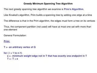
Greedy Algorithm
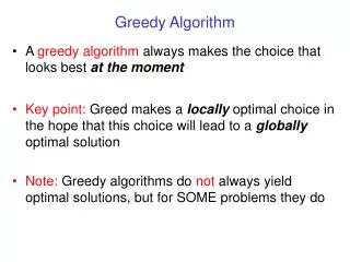
Greedy Algorithm. A greedy algorithm always makes the choice that looks best at the moment Key point: Greed makes a locally optimal choice in the hope that this choice will lead to a globally optimal solution

Greedy Algorithm
E N D
Presentation Transcript
Greedy Algorithm • A greedy algorithm always makes the choice that looks best at the moment • Key point: Greed makes a locally optimal choice in the hope that this choice will lead to a globally optimal solution • Note: Greedy algorithms do not always yield optimal solutions, but for SOME problems they do
Greed • When do we use greedy algorithms? • When we need a heuristic (e.g., hard problems like the Traveling Salesman Problem) • When the problem itself is “greedy” • Greedy Choice Property (CLRS 16.2) • Optimal Substructure Property (shared with DP) (CLRS 16.2) • Examples: • Minimum Spanning Tree (Kruskal’s algorithm) • Optimal Prefix Codes (Huffman’s algorithm)
Elements of the Greedy Algorithm • Greedy-choice property: “A globally optimal solution can be arrived at by making a locally optimal (greedy) choice.” • Must prove that a greedy choice at each step yields a globally optimal solution • Optimal substructure property: “A problem exhibits optimal substructure if an optimal solution to the problem contains within it optimal solutions to subproblems. This property is a key ingredient of assessing the applicability of greedy algorithm and dynamic programming.”
Proof of Kruskal’s Algorithm • Basis: |T| = 0, trivial. • Induction Step: T is promising by I.H., so it is a subgraph of some MST, call it S. Let ei be the smallest edge in E, s.t. T{ei} has no cycle, eiT. • If eiS, we’re done. • Suppose eiS, then S’ = S {ei} has a unique cycle containing ei, and all other arcs in cycle ei (because S is an MST!) • Call the cycle C. Observe that C with ei cannot be in T, because T {ei} is acyclic (because Kruskal adds ei)
ej ei Proof of Kruskal’s Algorithm • Then C must contains some edge ej s.t.ejS, and we also know c(ej)c(ei). • Let S’ = S {ei} \ {ej} • S’ is an MST, so T{ei} is promising
Greedy Algorithm: Huffman Codes • Prefix codes • one code per input symbol • no code is a prefix of another • Why prefix codes? • Easy decoding • Since no codeword is a prefix of any other, the codeword that begins an encoded file is unambiguous • Identify the initial codeword, translate it back to the original character, and repeat the decoding process on the remainder of the encoded file
Greedy Algorithm: Huffman Codes • Huffman coding • Given: frequencies with which with which source symbols (e.g., A, B, C, …, Z) appear in a message • Goal is to minimize the expected encoded message length • Create tree (leaf) node for each symbol that occurs with nonzero frequency • Node weights = frequencies • Find two nodes with smallest frequency • Create a new node with these two nodes as children, and with weight equal to the sum of the weights of the two children • Continue until have a single tree
A E G I M N O R S T U V Y Blank 1 5 7 9 13 14 15 18 19 20 21 22 24 Frequency: 1 3 2 2 1 2 2 2 2 1 1 1 1 3 • Place the elements into minimum heap (by frequency). • Remove the first two elements from the heap. • Combine these two elements into one. • Insert the new element back into the heap. • Note: circle for node, rectangle for weight (= frequency) Greedy Algorithm: Huffman Codes • Example:
4 4 2 N 4 T U 2 2 2 2 2 2 2 2 A A A V A V T T Y M M Y M U M U Greedy Algorithm: Huffman Codes Step 1: Step 2: Step 3: Step 4:
4 4 4 4 2 2 N N T T U U 2 4 4 4 2 2 2 S V A A O V O R M G R M Y Y Greedy Algorithm: Huffman Codes Step 5: Step 6:
7 4 4 4 4 2 2 N N T T U U 2 5 2 2 4 2 4 4 5 4 S S A I O V O I A V G Y M E G E R R Y M Greedy Algorithm: Huffman Codes Step 7 Step 8
15 9 8 7 4 4 2 N T U 5 2 4 4 2 A S I O V Y M G E R Greedy Algorithm: Huffman Codes • Step 9
24 0 15 1 9 8 7 4 4 0 1 0 1 2 N 0 0 1 0 1 0 1 1 T U 0 0 1 0 1 4 4 2 5 2 1 0 1 0 1 0 S V O A I E M G Y R Greedy Algorithm: Huffman Codes Finally: • Note that the 0’s (left branches) and 1’s (right branches) give the code words for each symbol
T y x a b Proof That Huffman’s Merge is Optimal • Let T be an optimal prefix-code tree in which a, b are siblings at deepest level, L(a) = L(b) • Suppose that x, y are two other nodes that are merged by the Huffman algorithm • x, y have lowest weights because Huffman chose them • WLOG w(x) £w(a), w(y) £ w(b); L(a) = L(b) L(x), L(y) • Swap a and x: cost difference between T and new T’ is • w(x)L(x) + w(a)L(a) – w(x)L(a) – w(a)L(x) = (w(a) – w(x))(L(a) – L(x)) // both factors non-neg 0 • Similar argument for b, y Huffman choice also optimal
Dynamic Programming • Dynamic programming: Divide problem into overlapping subproblems; recursively solve each in the same way. • Similar to DQ, so what’s the difference: • DQ partition the problem into independent subproblems. • DP breaking it into overlapping subproblems, that is, when subproblems share subproblems. • So DP saves work compared with DQ by solving every subproblems just once ( when subproblems are overlapping).
Elements of Dynamic Programming • Optimal substructure: A problem exhibits optimal substructure if an optimal solution to the problem contains within it optimal solutions to subproblems. Whenever a problem exhibits optimal substructure, it is a good clue that DP might apply.(a greedy method might apply also.) • Overlapping subproblems: A recursive algorithm for the problem solves the same subproblems over and over, rather than always generating new subproblems.
Dynamic Programming: Matrix Chain Product • Matrix-chain multiplication problem: Give a chain of n matrices A1, A2, …, An to be multiplied, how to get the product A1 A2 …An. with minimum number of scalar multiplications. • Because of the associative law of matrix multiplication, there are many possible orderings to calculate the product for the same matrix chain: • Only one way to multiply A1 A2 • Best way for triple: Cost (A1 , A2) +Cost((A1 A2)A3) or Cost (A2 , A3) +Cost(A1 (A2A3)).
5 3 3 10 3 10 Dynamic Programming: Matrix Chain Product • How do we build bottom-up? • From last example: • Best way for triple: Cost (A1 , A2) +Cost((A1 A2)A3) or Cost (A2 , A3) +Cost(A1 (A2A3)). • Save the best solutions for contiguous groups of Ai. • Cost of ( ij )( j k) is ijk. E.g., Each of 3•10 entries requires 5 multiplies (+ 4 adds)
d1 dk dkdn+1 Dynamic Programming: Matrix Chain Product • Cost of final multiplication? A1 • A2 • A3 •… •Ak-1 • Ak •…•An. • Each of these subproblems can be solved optimally – just look in the table
Dynamic Programming: Matrix Chain Product • FORMULATION: • Table entries aij, 1 i j n, where aij = optimal solution = min #multiplications for Ai • Ai+1 •… •Aj-1 • Ak • • We want aij to fill the table. • Let dimensions be given by vectordi, 1 i n+1, i.e., Ai is didi+1
Dynamic Programming: Matrix Chain Product • Build Table: Diagonal S contains aij with j - i = S. • S = 0: aij =0, i=1, 2, …, n S = 1: ai, i+1 = di di+1di+2, i=1, 2, …, n-1 1 S n: ai, i+s= (ai, k+ ak+1, i+s + di dkdi+s ) • Example: (Brassard/Bratley) 4 matrices, d = (13, 5, 89, 3, 34) S = 1: a12 =5785 a23=1335 a34 =9078
Dynamic Programming: Matrix Chain Product S = 2: a13 = min(a11+ a23 + 13•5•3, a12+ a33+13•89•3) = 1530 a24 = min(a22+ a34 + 5•89•34, a23+ a44 +5•3•34) = 1845 S = 3: a14 = min( {k=1} a11 + a24 + 13•5•34, {k=2} a12 + a34 + 13•89•34, {k=3} a13 + a44 + 13•3•34) = 2856 (note: max cost is 54201 multiplies) • Complexity:S>0, choose among S choices for each of n-S elements in diagonal, so runtime is (n3). Proof: åi = 1 to n i(n-i) = åi = 1 to n (ni – i2) = n(n(n+1)/2) – (n(n+1)(2n+1)/6) = (n3)
Dynamic Programming: Longest Common Subsequence • Longest Common Subsequence: Give two strings [a1 a2… am] and [b1 b2… bn], what is the largest value P such that: For indices 1 i1 i2 … ip m, and 1 j1 j2 … jp n, We have aix= bjx, for 1 x P • Example: So P = 4, i = {1, 2, 3, 5}, j = {3, 4, 5, 6} b a a b a c b a c b a a a
Dynamic Programming: Longest Common Subsequence Let L(k, l) denote length of LCS for [a1 a2… ak] and [b1 b2… bl]. Then we have facts: • L(p, q) L(p-1, q-1). • L(p, q) = L(p-1, q-1) + 1 if ap = bq when ap and bq are both in LCS. • L(p, q) L(p-1, q) when ap is not in LCS. • L(p, q) L(p, q-1) when bq is not in LCS.
Dynamic Programming: Longest Common Subsequence • ALGORITHM: for i = 1 to m for j = 1 to n if ai = bj then L(i, j) = L(i-1, j-1) + 1 else L(i, j) = max{L(i, j-1), L(i-1, j)} • Time complexity:(n2).
Dynamic Programming: Knapsack • The problem: The knapsack problem is a particular type of integer program with just one constraint: Each item that can go into the knapsack has a size and a benefit. The knapsack has a certain capacity. What should go into the knapsack so as to maximize the total benefit? • Hint: Recall shortest path method. Define Fk(y) = max (0kn) with (0yb) • Then, what is Fk(y)? Max value possible using only first k items when weight limit is y.
Kth item not used Kth item used once Dynamic Programming: Knapsack • B.C.’s: 1. F0(y) = 0 y no items chosen 2. Fk(0) = 0 k weight limit = 0 3. F1(y) = y/w1v1 Generally speaking: Fk(y) = max{Fk-1(y), Fk(y-wk)+vk} • Then we could build matrix: use entries above, here is an example:
Dynamic Programming: Knapsack • Example: k=4, b=10, y=#pounds, k=#item types allowed v1=1 w1=2; v2=3 w2=3; v3=5 w3=4; v4=9 w4=7 Fk(y) = max{Fk-1(y), Fk(y-wk)+vk} Fk(y) nb table:
Dynamic Programming: Knapsack • Note: 12 = max(11, 9+ F4(3))=max(11,9+3)=12 • What is missing here? (Like in SP, we know the SP’s cost, but we don’t know SP itself…) • So, we need another table? i(k,j) = max index such that item type j is used in Fk(y), i.e., i(k,y)=j xj1; xq=0 q>j • B.C.’s: i(1,y) =0 if F1(y) = 0 i(1,y) =0 if F1(y) 0 • General:
Dynamic Programming: Knapsack • Trace Back: if i(k,y) =q, use item q once, check i(k,y-q). • Example: • E.g. F4(10) = 12. i(4,10)=4 4th item used once
Dynamic Programming: Knapsack i(4, 10 - w4) =i(4,3)=2 2nd item used once i(4, 3 – w2) =i(4,0)=0 done • Notice i(4,8)=3 don’t use most valuable item.