Greedy algorithm
Greedy algorithm. 叶德仕 yedeshi@zju.edu.cn. Greedy algorithm’s paradigm. Algorithm is greedy if it builds up a solution in small steps it chooses a decision at each step myopically to optimize some underlying criterion Analyzing optimal greedy algorithms by showing that:


Greedy algorithm
E N D
Presentation Transcript
Greedy algorithm 叶德仕 yedeshi@zju.edu.cn
Greedy algorithm’s paradigm • Algorithm is greedyif • it builds up a solution in small steps • it chooses a decision at each step myopically to optimize some underlying criterion • Analyzing optimal greedy algorithms by showing that: • in every step it is not worse than any other algorithm, or • every algorithm can be gradually transformed to the greedy one without hurting its quality
Interval scheduling • Input: set of intervals on the line, represented by pairs of points (ends of intervals). In another word, the ith interval, starts at time si and finish at fi. • Output: finding the largest set of intervals such that none two of them overlap. Or the maximum number of intervals that without overlap. • Greedy algorithm: • Select intervals one after another using some rule
Rule 1 • Select the interval which starts earliest (but not overlapping the already chosen intervals) • Underestimated solution! OPT #4 Algorithm #1
Rule 2 • Select the interval which is shortest (but not overlapping the already chosen intervals) • Underestimated solution! OPT#2 Algorithm #1
Rule 3 • Select the interval with the fewest conflicts with other remaining intervals (but still not overlapping the already chosen intervals) • Underestimated solution! OPT#4 Algorithm #3
Rule 4 • Select the interval which ends first (but still not overlapping the already chosen intervals) • Quite a nature idea: we ensure that our resource become free as soon as possible while still satisfying one request • Hurray! Exact solution!
f1 smallest Algorithm #3
Analysis - exact solution • Algorithm gives non-overlapping intervals: • obvious, since we always choose an interval which does not overlap the previously chosen intervals • The solution is exact: • Let Abe the set of intervals obtained by the algorithm, • and OPTbe the largest set of pairwise non-overlapping intervals. • We show that Amust be as large as OPT
Analysis – exact solution cont. • Let and be sorted. By definition of OPT we have k ≤ m • Fact: for every i ≤ k, Aifinishes not later than Bi. • Pf. by induction. • For i = 1 by definition of a step in the algorithm. • Suppose that Ai-1 finishes not later than Bi-1.
Analysis con. • From the definition of a step in the algorithm we get that Aiis the first interval that finishes after Ai-1 and does not verlap it. • If Bifinished before Aithen it would overlap some of the previous A1,…, Ai-1 and • consequently - by the inductive assumption - it would overlap Bi-1, which would be a contradiction. Bi-1 Bi Ai Ai-1
Analysis con. • Theorem:A is the exact solution. • Proof: we show that k = m. • Suppose to the contrary that k < m. We have that Akfinishes not later than Bk • Hence we could add Bk+1 to A and obtain bigger solution by the algorithm-contradiction Bk-1 Bk Bk+1 Ak Ak-1
Time complexity • Sorting intervals according to the right-most ends • For every consecutive interval: • If the left-most end is after the right-most end of the last selected interval then we select this interval • Otherwise we skip it and go to the next interval • Time complexity: O(n log n + n) = O(n log n)
Planning of schools • A collection of towns. We want to plan schools in towns. • Each school should be in a town • No one should have to travel more than 30 miles to reach one of them. Edge: towns no far than 30 miles
Set cover • Input. A set of elements B, sets • Output. A selection of the Siwhose union is B. • Cost. Number of sets picked.
Greedy • Greedy: first choose a set that covers the largest number of elements. • example: place a school at town a, since this covers the largest number of other towns. Greedy #4 OPT #3
Upper bound • Theorem. Suppose B contains n elements that the optimal cover consist of k sets. Then the greedy algorithm will use at most k ln n sets. • Pf. Let nt be the number of elements still not covered after t iterations of the greedy algorithm (n0=n). Since these remaining elements are covered by the optimal k sets, there must be some set with at least nt /kof them. Therefore, the greedy algorithm will ensure that
Upper bound con. • Then , since for all x, with equality if and only if x=0. • Thus • At t=k ln n, therefore, nt is strictly less than ne-ln n =1, which means no elements remains to be covered. • Consequently, the approximation ratio is at most ln n
Exercise • Knapsack problem
Marking Changes • Goal. Given currency denominations in HK: 1, 2, 5, 10, 20, 50, 100, 500, and 1000, devise a method to pay amount to customer using fewest number of notes/coins. • Cashier's algorithm. At each iteration, add note/coin of the largest value that does not take us past the amount to be paid.
Optimal Offline Caching • Caching. • Cache with capacity to store k items. • Sequence of m item requests d1, d2, …, dm. • Cache hit: item already in cache when requested. • Cache miss: item not already in cache when requested: must bring requested item into cache, and evict some existing item, if full. (It also refers to the operation of bringing an item into cache.) • Goal. Eviction schedule that minimizes number of cache misses. • Ex: k = 2, initial cache = ab, requests: a, b, c, b, c, a, a, b. • Optimal eviction schedule: 2 cache misses. a a b b a b c c b b c b c c b a a b a a b b a b cache requests
Optimal Offline Caching: Farthest-In-Future • Farthest-in-future. Evict item in the cache that is not requested until farthest in the future. • Theorem. [Bellady, 1960s] FF is optimal eviction schedule. • Pf. Algorithm and theorem are intuitive; proof is subtle. current cache: a b c d e f future queries: g a b c e d a b b a c d e a f a d e f g h ... eject this one cache miss
Minimum spanning tree Input: weighted graph G = (V,E) • every edge in E has its positive weight Output: finding the spanning tree such that the sum of weights is not bigger than the sum of weights of any other spanning tree Spanning tree: subgraph with • no cycle, and • connected (every two nodes in V are connected by a path) 2 2 2 1 1 1 1 1 1 2 2 2 3 3 3
Properties of minimum spanning trees MST Spanning trees: • n nodes • n - 1 edges • at least 2 leaves (leaf - a node with only one neighbor) MST cycle property: • After adding an edge we obtain exactly one cycle and all the edges from MST in this cycle have no bigger weight than the weight of the added edge 2 2 1 1 1 1 2 2 3 3 cycle
Optimal substructures MST T: (Other edges of G are not shown.)
Optimal substructures u MST T: (Other edges of G are not shown.) v Remove any edge (u, v) ∈ T.
Optimal substructures T1 MST T: (Other edges of G are not shown.) T2 Remove any edge (u, v) ∈ T. Then, T is partitioned into two subtrees T1 and T2.
Optimal substructures T1 MST T: (Other edges of G are not shown.) T2 Remove any edge (u, v) ∈ T. Then, T is partitioned into two subtrees T1 and T2. Theorem. The subtree T1 is an MST of G1 = (V1, E1), the subgraph of G induced by the vertices of T1: V1 = vertices of T1, E1 = { (x, y) ∈ E : x, y ∈ V1 }. Similarly for T2.
Proof of optimal substructure • Proof. Cut and paste: • w(T) = w(u, v) + w(T1) + w(T2). • If T1′ were a lower-weight spanning tree than T1 for G1, then T′ = {(u, v)} ∪ T1′ ∪ T2 • would be a lower-weight spanning tree than T for G.
Do we also have overlapping subproblems? • Yes. • Great, then dynamic programming may work! • Yes, but MST exhibits another powerful property which leads to an even more efficient algorithm.
Crucial observation about MST Consider sets of nodes A and V - A Let F be the set of edges between A and V - A Let abe the smallest weight of an edge from F Theorem: Every MST must contain at least one edge of weight a from set F A A 2 2 1 1 1 1 2 2 3 3
Proof of the observation Let e be the edge in F with the smallest weight - for simplicity assume that there is unique such edge. Suppose to the contrary that e is not in some MST. Choose one such MST. Add e to MST - obtain the cycle, where e is (among) smallest weights. Since two ends of e are in different sets A and V - A, there is another edge f in the cycle and in F. Remove f from the tree (with added edge e) - obtain a spanning tree with the smaller weight (since f has bigger weight than e). This is a contradiction with MST. A A 2 2 1 1 1 1 2 2 3 3
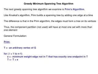
Greedy algorithm finding MST Kruskal’s algorithm: • Sort all edges according to the weights in non-increasing order • Choose n - 1 edges one after another as follows: • If a new added edge does not create a cycle with previously selected then we keep it in (partial) MST, otherwise we remove it Remark: we always have a partial forest 2 2 2 1 1 1 1 1 1 2 2 2 3 3 3
Greedy algorithm finding MST Prim’s algorithm: • Select a node as a root arbitrarily • Choose n - 1 edges one after another as follows: • Look on all edges incident to the currently build (partial) tree and which do not create a cycle in it, and select one which has the smallest weight Remark: we always have a connected partial tree root 2 2 2 1 1 1 1 1 1 2 2 2 3 3 3
Example of Prim A 12 6 9 5 V - A 8 14 7 15 3 10
Example of Prim A 12 6 9 5 V - A 8 14 7 15 3 10
Example of Prim A 12 6 9 5 7 V - A 8 14 7 15 0 3 10
Example of Prim A 12 6 9 5 7 V - A 8 14 7 15 0 3 10
Example of Prim A 12 6 9 5 5 7 V - A 8 14 7 15 0 3 10
Example of Prim 6 A 12 6 9 5 5 7 V - A 8 14 7 15 0 3 10
Example of Prim 6 A 12 6 9 5 5 7 V - A 8 14 7 15 0 3 8 10
Example of Prim 6 A 12 6 9 5 5 7 V - A 8 14 7 15 0 3 8 10
Example of Prim 6 A 12 6 9 5 5 7 V - A 8 14 7 3 15 0 3 8 10
Example of Prim 6 A 12 6 9 5 5 7 9 V - A 8 14 7 3 15 0 3 8 10
Example of Prim 6 A 12 6 9 5 5 7 9 V - A 8 14 7 3 15 15 0 3 8 10
Example of Prim 6 A 12 6 9 5 5 7 9 V - A 8 14 7 3 15 15 0 3 8 10
Why the algorithms work? Follows from the crucial observation Kruskal’s algorithm: • Suppose we add edge {v,w}. This edge has the smallest weight among edges between the set of nodes already connected with v (by a path in selected subgraph) and other nodes. Prim’s algorithm: • Always chooses an edge with the smallest weight among edges between the set of already connected nodes and free nodes.
Time complexity There are implementations using • Union-find data structure (Kruskal’s algorithm) • Priority queue (Prim’s algorithm) achieving time complexity O(m log n) where n is the number of nodes and m is the number of edges
Best of MST • Best to date: • Karger, Klein, and Tarjan [1993]. • Randomized algorithm. • O(V + E) expected time.
Conclusions Greedy algorithms for finding minimum spanning tree in a graph, both in time O(m log n) : • Kruskal’s algorithm • Prim’s algorithm Remains to design the efficient data structures!