Greedy Algorithm, Dynamic Programming Algorithm
計概補充. Greedy Algorithm, Dynamic Programming Algorithm. 蔡文能 CSIE.NCTU.EDU.TW. Agenda. Complexity: Big O, Big Omega, Big Theta Knapsack problem Greedy Algorithm Making Change problem Knapsack problem Dynamic Programming (DP) DP vs. Divide-and-Conquer Greedy vs. Dynamic Programming


Greedy Algorithm, Dynamic Programming Algorithm
E N D
Presentation Transcript
計概補充 Greedy Algorithm,Dynamic ProgrammingAlgorithm 蔡文能 CSIE.NCTU.EDU.TW
Agenda • Complexity: Big O, Big Omega, Big Theta • Knapsack problem • Greedy Algorithm • Making Change problem • Knapsack problem • Dynamic Programming (DP) • DP vs. Divide-and-Conquer • Greedy vs. Dynamic Programming • Quick Sort, merge Sort • C++ STL sort( ), java.util.Arrays.sort( )
Asymptotic Upper Bound (Big O) • f(n) c g(n) for all nn0 • g(n) is called an • asymptotic upper bound of f(n). • We write f(n)=O(g(n)) • It reads f(n) equals big oh of g(n). c g(n) f(n) n0
Asymptotic Lower Bound (Big Omega) • f(n) c g(n) for all nn0 • g(n) is called an • asymptotic lower bound of f(n). • We write f(n)=(g(n)) • It reads f(n) equals big omega of g(n). f(n) c g(n) n0
Asymptotically Tight Bound (Big Theta) • f(n) = O(g(n)) and f(n) = (g(n)) • g(n) is called an • asymptotically tight bound of f(n). • We write f(n)=(g(n)) • It reads f(n) equals theta of g(n). c2 g(n) f(n) c1 g(n) n0
Algorithm types • Algorithm types we will consider include: • Simple recursive algorithms • Backtracking algorithms • Greedy algorithms • Divide and conquer algorithms • Dynamic programming algorithms • Branch and bound algorithms • Brute force algorithms • Randomized algorithms
Knapsack Problem • Knapsack Problem: Given n items, with ith item worth vi dollars and weighing wi pounds, a thief wants to take as valuable a load as possible, but can carry at most W pounds in his knapsack. • The 0-1 knapsack problem: Each item is either taken or not taken (0-1 decision). • The fractional knapsack problem: Allow to take fraction of items. (較簡單) • Exp: = (60, 100, 120), = (10, 20, 30), W = 50 • Greedy solution by taking items in order of greatest value per pound is optimal for the fractional version, but not for the 0-1 version. • The 0-1 knapsack problem is NP-complete, but can be solved in O(nW) time by Dynamic Programming. (A polynomial-time DP??)
The Fractional Knapsack Problem • Given: A set S of n items, with each item i having • bi - a positive benefit • wi - a positive weight • Goal: Choose items with maximum total benefit but with weight at most W. • If we are allowed to take fractional amounts, then this is the fractional knapsack problem. • In this case, we let xi denote the amount we take of item i • Objective: maximize • Constraint:
The Fractional Knapsack Algorithm • Greedy choice: Keep taking item with highest value (benefit to weight ratio) • Since • Run time: O(n log n). Why? • Correctness: Suppose there is a better solution • there is an item i with higher value than a chosen item j, but xi<wi, xj>0 and vj<vi • If we substitute some j with i, we get a better solution • How much of i: min{wi-xi, xj} • Thus, there is no better solution than the greedy one AlgorithmfractionalKnapsack(S,W) Input:set S of items w/ benefit biand weight wi; max. weight WOutput:amount xi of each item i to maximize benefit w/ weight at most W for each item i in S xi 0 vi bi / wi{value} w 0 {total weight} whilew < W remove item i w/ highest vi xi min{wi , W - w} w w + min{wi , W - w}
0-1 Knapsack problem (1/5) • Given a knapsack with maximum capacity W, and a set S consisting of n items • Each item i has some weight wi and benefit value bi(all wi , biand W are integer values) • Problem: How to pack the knapsack to achieve maximum total value of packed items?
Weight Benefit value wi bi Items 3 2 3 4 W = 20 5 4 5 8 9 10 0-1 Knapsack problem (2/5) This is a knapsack Max weight: W = 20
0-1 Knapsack problem (3/5) • Problem, in other words, is to find • The problem is called a “0-1” Knapsack problem, because each item must be entirely accepted or rejected. • Another version of this problem is the “Fractional Knapsack Problem”, where we can take fractions of items.
0-1 Knapsack problem (4/5) Let’s first solve this problem with a straightforward algorithm (Brute-force) • Since there are n items, there are 2npossible combinations of items. • We go through all combinations and find the one with the most total value and with total weight less or equal to W. • Running time will be O(2n)
Brute force ? • Brute = Beast 野獸 • Brute 是個英雄(Marcus Junius Brutus ),出現在莎士比亞擷取羅馬歷史上西元前44年凱撒遇刺事件所寫描述一個英雄 墜落的悲劇《凱撒大帝》。貴族世家後 代的Brute 原為凱撒忠臣,因凱撒獨裁憂心羅馬前途決定刺殺凱撒。 • Brutus 刺殺凱撒大帝後自殺之前留下一句名言:「並非我愛凱撒較少,而是我愛羅馬更多。」 In Shakespeare's "Julius Caesar," he is called Brute, and not Brutus, because "Brute" is in the Vocative Case in Latin. • 1929年漫畫家西格(Elzie Segar)創作連載漫畫大力水手卜派(PopEye the Sailor) • 1933 Fleischer Studios 改編為戲劇, Brute Bluto是 Popeye的死對頭! 1961年更搬上電視卡通 (cartoon) !
0-1 Knapsack problem (5/5) • Can we do better? • Yes, with an algorithm based on Dynamic programming • We need to carefully identify the subproblems Key point: If items are labeled 1..n, then a subproblem would be to find an optimal solution for Sk = {items labeled 1, 2, .. k}
Algorithm types • Algorithm types we will consider include: • Simple recursive algorithms • Backtracking algorithms • Greedy algorithms • Divide and Conquer algorithms • Dynamic programming algorithms • Branch and bound algorithms • Brute force algorithms • Randomized algorithms
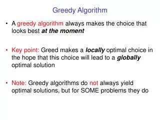
The greedy method is a general algorithm design paradigm, built on the following elements: configurations: different choices, collections, or values to find objective function: a score assigned to configurations, which we want to either maximize or minimize A greedy algorithm always makes the choice that looks best at the moment. (時到時擔當, 沒米再煮蕃薯塊湯) Top-down algorithmic structure With each step, reduce problem to a smaller problem It works best when applied to problems with the greedy-choice property: a globally-optimal solution can always be found by a series of local improvements from a starting configuration. The Greedy Method Technique The greedy method cannot always find an optimal solution!
Problem: A dollar amount to reach and a collection of coin amounts to use to get there. Configuration: A dollar amount yet to return to a customer plus the coins already returned Objective function:Minimize number of coins returned. Greedy solution: Always return the largest coin you can Example 1: Coins are valued $.32, $.08, $.01 Has the greedy-choice property, since no amount over $.32 can be made with a minimum number of coins by omitting a $.32 coin (similarly for amounts over $.08, but under $.32). Coin Changing problem Coins in USA: 1 ¢ 5 ¢ 10 ¢ 25 ¢ 50 ¢
Greedy Algorithm for Coin Changing problem This algorithm makes change for an amount A using coins of denominations denom[1] > denom[2] > ··· > denom[n] = 1. Input Parameters: denom, A Output Parameters: None greedy_coin_change(int denom[], int A) { i = 1 while (A > 0) { c = A/denom[ i ] println(“use ” + c + “ coins of denomination ” + denom[i]) A = A - c * denom[i] i = i + 1 } }
Suppose there are unlimited quantities of coins of each denomination. What property should the denominations c1, c2, …, ck have so that the greedy algorithm always yields an optimal solution? Consider this example: Example 2: Coins are valued $.30, $.20, $.05, $.01 Does not have greedy-choice property, since $.40 is best made with two $.20’s, but the greedy solution will pick three coins (which ones?) Question ? The greedy method cannot always find an optimal solution!
Consider the Coin set for examples • For the following examples, we will assume coins in the following denominations: 1¢ 5¢ 10¢ 21¢ 25¢ • We’ll use 63¢ as our goal • This example is taken from:Data Structures & Problem Solving using Java by Mark Allen Weiss The greedy method cannot always find an optimal solution!
(1) A simple solution • We always need a 1¢ coin, otherwise no solution exists for making one cent • To make K cents: • If there is a K-cent coin, then that one coin is the minimum • Otherwise, for each value i < K, • Find the minimum number of coins needed to make i cents • Find the minimum number of coins needed to make K - i cents • Choose the i that minimizes this sum • This algorithm can be viewed as divide-and-conquer, or as brute force • This solution is very recursive • It requires exponential work • It is infeasible to solve for 63¢
(2) Another solution • We can reduce the problem recursively by choosing the first coin, and solving for the amount that is left • For 63¢: • One 1¢ coin plus the best solution for 62¢ • One 5¢ coin plus the best solution for 58¢ • One 10¢ coin plus the best solution for 53¢ • One 21¢ coin plus the best solution for 42¢ • One 25¢ coin plus the best solution for 38¢ • Choose the best solution from among the 5 given above • Instead of solving 62 recursive problems, we solve 5 • This is still a very expensive algorithm
(3) A dynamic programming solution • Idea: Solve first for one cent, then two cents, then three cents, etc., up to the desired amount • Save each answer in an array ! • For each new amount N, compute all the possible pairs of previous answers which sum to N • For example, to find the solution for 13¢, • First, solve for all of 1¢, 2¢, 3¢, ..., 12¢ • Next, choose the best solution among: • Solution for 1¢ + solution for 12¢ • Solution for 2¢ + solution for 11¢ • Solution for 3¢ + solution for 10¢ • Solution for 4¢ + solution for 9¢ • Solution for 5¢ + solution for 8¢ • Solution for 6¢ + solution for 7¢
Example using Dynamic Programming • Suppose coins are 1¢, 3¢, and 4¢ • There’s only one way to make 1¢ (one coin) • To make 2¢, try 1¢+1¢ (one coin + one coin = 2 coins) • To make 3¢, just use the 3¢ coin (one coin) • To make 4¢, just use the 4¢ coin (one coin) • To make 5¢, try • 1¢ + 4¢ (1 coin + 1 coin = 2 coins) • 2¢ + 3¢ (2 coins + 1 coin = 3 coins) • The first solution is better, so best solution is 2 coins • To make 6¢, try • 1¢ + 5¢ (1 coin + 2 coins = 3 coins) • 2¢ + 4¢ (2 coins + 1 coin = 3 coins) • 3¢ + 3¢ (1 coin + 1 coin = 2 coins) – best solution • Etc.
How good is the algorithm? • The first algorithm is recursive, with a branching factor of up to 62 • Possibly the average branching factor is somewhere around half of that (31) • The algorithm takes exponential time, with a large base • The second algorithm is much better—it has a branching factor of 5 • This is exponential time, with base 5 • The dynamic programming algorithm is O(N*K), where N is the desired amount and K is the number of different kinds of coins
Dynamic Programming (DP) ? • Like divide-and-conquer, solve problem by combining the solutions to sub-problems. • Differences between divide-and-conquer and DP: • Independent sub-problems, solve sub-problems independently and recursively, (so same sub(sub)problems solved repeatedly) • Sub-problems are dependent, i.e., sub-problems share sub-sub-problems, every sub(sub)problem solved just once, solutions to sub(sub)problems are stored in a table and used for solving higher level sub-problems. • DP reduces computation by • Solving subproblems in a bottom-up fashion. • Storing solution to a subproblem the first time it is solved. • Looking up the solution when subproblem is encountered again.
Fibonacci sequence (1/4) • Fibonacci sequence: 1 , 1 , 2 , 3 , 5 , 8 , 13 , 21 , … Fi = 1if i==1 or i == 2 (assume F0= 0) Fi = Fi-1 + Fi-2 if i 3 • Solved by a recursive program: • Much replicated computation is done. • It should be solved by a simple loop.
Recursive logic: F1 = F2 = 1 If i > 2 then Fi = Fi-1 + F i-2 Directly translates into a recursive algorithm F: F(i) { if (i = 1) or (i = 2) x 1 else x F(i-1) + F(i-2) return x } F’s call tree is exponential;F is recomputed many times for the same input value! Fibonacci Sequence (2/4) • We can speed things up by storing output values of F in an array AF F(i) { if (AF != NULL) return AF if (i = 1) or (i = 2) x 1 else x F(i-1) + F(i-2) AF x return x } • Since there are n cells in AF and each cell takes O(1) time to compute, this is O(n)!
Fibonacci Sequence (3/4) • The final algorithm is: Fib(n) { AF new array of n int’s for (i = 1 to n) { if (i = 1) or (i = 2) x 1 else x F(i-1) + F(i-2) AF[i] x } return AF[n] } • This is a dynamic programming algorithm! • We have sped things up by storing output values of F in an array AF F(i) { if (AF != NULL) return AF if (i = 1) or (i = 2) x 1 else x F(i-1) + F(i-2) AF x return x } • But we don’t need recursion at all, just a loop through AF!
Fibonacci Sequence (4/4) using Dynamic programming • Dynamic programming calculates from bottom to top. (bottom-up) • Values are stored for later use. • This reduces repetitive calculation. Pascal Triangle ?
Application domain of DP • Optimization problem: find a solution with optimal (maximum or minimum) value. • Anoptimal solution, not the optimal solution, since may more than one optimal solution, any one is OK. • Dynamic Programming is an algorithm design method that can be used when the solution to a problem may be viewed as the result of a sequence of decisions DP : Dynamic programming
Typical steps of DP • Characterize the structure of an optimal solution. • Recursively define the value of an optimal solution. • Compute the value of an optimal solution in a bottom-up fashion. • Compute an optimal solution from computed/stored information. DP : Dynamic programming
Comparison with Divide-and-Conquer • Divide-and-conquer algorithms split a problem into separate subproblems, solve the subproblems, and combine the results for a solution to the original problem • Example: Quicksort • Example: Mergesort • Example: Binary search • Divide-and-Conquer algorithms can be thought of as top-downalgorithms • In contrast, a dynamic programming algorithm proceeds by solving small problems, then combining them to find the solution to larger problems • Dynamic programming can be thought of asbottom-up Divide-and-Conquer 分割征服 ;各個擊破;拆解
Divide and Conquer • Divide the problem into a number of sub-problems (similar to the original problem but smaller); • Conquer the sub-problems by solving them recursively (if a sub-problem is small enough, just solve it in a straightforward manner (base case).) • Combine the solutions to the sub-problems into the solution for the original problem
Divide and Conquer example : Merge Sort • Divide the n-element sequence to be sorted into two subsequences of n/2 element each • Conquer: Sort the two subsequences recursively using merge sort • Combine:merge the two sorted subsequences to produce the sorted answer • Note: during the recursion, if the subsequence has only one element, then do nothing.
Comparison with Greedy • Common: optimal substructure • Optimal substructure: An optimal solution to the problem contains within its optimal solutions to subproblems. • E.g., if A is an optimal solution to S, then A' = A - {1} is an optimal solution to S' = {iS: sif1}. • Difference: greedy-choice property • Greedy: A global optimal solution can be arrived at by making a locally optimal choice. • Dynamic programming needs to check the solutions to subproblems. • DP can be used if greedy solutions are not optimal. The greedy method cannot always find an optimal solution!
Greedy vs. Dynamic Programming • The knapsack problem is a good example of the difference. • 0-1 knapsack problem: not solvable by greedy. • n items. • Itemi is worth $vi, weighswipounds. • Find a most valuable subset of items with total weight ≤ W. • Have to either take an item or not take it—can’t take part of it. • Fractional knapsack problem:solvable by greedy • Like the 0-1 knapsack problem, but can take fraction of an item. • Both have optimal substructure. • But the fractional knapsack problem has the greedy-choice property, and the 0-1 knapsack problem does not. • To solve the fractional problem, rank items by value/weight:vi/ wi. • Letv i / wi≥ vi+1/ wi+1for all i . The greedy method cannot always find an optimal solution!
Divide-and-Conquer in Sorting • Mergesort • O(n log n) always, but O(n) storage • Quick sort • O(n log n) average, O(n^2) worst in time • O(log n) storage • Good in practice (when n >12) What is a Stable sort?
Quick sort is NOT Stable; But can implemented as Stable Quick Sort (1/6) • Algorithm quick_sort(array A, from, to) • Input: from - pointer to the starting position of array A • to - pointer to the end position of array A • Output: sorted array: A’ • 1. Choose any one element as the pivot; • 2. Find the first element a = A[i] larger than or equal to pivot from • A[from] to A[to]; • 3. Find the first element b = A[j] smaller than or equal to pivot from • A[to] to A[from]; • 4. If i < j then exchange a and b; • 5. Repeat step from 2 to 4 until j <= i; • 6. If from < j then recursive call quick_sort(A, from, j); • 7. If i < to then recursive call quick_sort(A, i, to);
Choose 5 as pivot Quick Sort (2/6) • Quick sort • main idea: • 1st step: 3 1 6 5 4 8 10 7 • 2nd step: 3 2 1 5 8 9 10 7 • 3rd step: 3 2 1 4 5 6 8 9 10 7 from to 9 2 j i 6 4 Smaller than any integer right to 5 greater than any integer left to 5
to from pivot pivot from to 1 3 8 7 6th step: 5 6 7 8 10 9 7th step: 7 8 10 9 8th step: 9 10 Quick Sort (3/6) • Quick sort • 4th step: 2 4 5 6 10 9 • 5th step: 1 2 3 4 5
Quick Sort (4/6) • public class QuickSorter { // Java function should be in a class • public static void sort (int[ ] a, int from, int to) { • if ((a == null) || (a.length < 2)) return; • int i = from, j = to; • int pivot = a[(from + to)/2]; • do { • while ((i < to) && (a[i] < pivot)) i++; • while ((j > from) && (a[j] >= pivot)) j--; • if (i < j) { int tmp =a[i]; a [i] = a[j]; a[j] = tmp;} • i++; j--; • }while (i <= j); exchange(a, i, (from+to)/2 ); /***/ • if (from < j) sort(a, from, j); • if (i < to) sort(a, i, to); } • }
3, 4, 6, 1, 10, 9, 5, 20, 19, 14, 12, 2, 15, 21, 13, 18, 17, 8, 16, 1 1, 12, 2, 15, 21, 13, 18, 17, 8, 16, 3, 4, 6, 1, 10, 9, 5, 20, 19, 14 j i 8, 14 1, 12, 2, 15, 21, 13, 18, 17, ,16, 19, 3, 4, 6, 1, 10, 9, 5, 20, i j 3, 4, 6, 1, 10, 9, 5, 8, 13 , 1, 12, 2,15, 21, 19, 18, 17, 20, 16, 14 i j 3, 4, 6, 1, 10, 9, 5, 8, 13, 1, 12, 2, 14, 21, 19, 18, 17, 20, 16, 15 14 i 3, 4, 6, 1, 10, 9, 5, 8, 13, 1, 12, 2 j Quick Sort (5/6)
Quick Sort (6/6) • void qsort (int a[ ], int from, int to) { • int n = to – from + 1; • if ( (n < 2) || (from >= to) ) return; • int k = (from + to)/2; int tmp =a[to]; a [to] = a[k]; a[k] = tmp; • int pivot = a[to]; // choose a[to] as the pivot • int i = from, j = to-1; • while(i < j ) { • while ((i < j) && (a[i] < pivot)) i++; • while ((i < j) && (a[j] >= pivot)) j--; • if (i < j) { tmp =a[i]; a [i] = a[j]; a[j] = tmp;} • }; • tmp =a[i]; a [i] = a[to]; a[to] = tmp; // exchange • if (from < i-1) qsort(a, from, i-1); • if (i < to) qsort(a, i+1, to); }
有大bugs的 quick sort 程式碼 //buga.c with Big BUG (quick sort) // 這sort程式有一個大 bug : // .. i 往右時可能會走過頭 ! j 往左時也可能會走過頭 ! // program 會在執行時當掉 ! Why? void sort( int left, int right, double x[ ]) { // 注意參數順序要與呼叫者相同 int i, j; double tmp; i = left; j = right+1; // i points to LEFT, j points to 最右的下一個 while( i<=j ) { // use left element as pivot do { i++; } while( x[i] >= x[left]); // Bug Bug Bug do { j--; } while ( x[j] <= x[left]); //Bug Bug Bug if(i<j) {tmp=x[i]; x[i]=x[j]; x[j]=tmp; } } tmp=x[j]; x[j]=x[left]; x[left]=tmp; if(left< j-1) sort(left, j-1, x); if(j+1 < right) sort(j+1, right, x); } // sort( )
有小bugs的 quick sort 程式碼 Hint: 修改紅色部份 //bugb.c with small BUG (quick sort) // 這sort程式有一個小 bug : (已經試著要 fix Big Bug) // .. i 往右時可能會走過頭 ! j 往左時也可能會走過頭 ! // Please try to fix it void sort( int left, int right, double x[ ]) { // use left element as pivot int i, j; double tmp; i = left; j = right+1; // i points to LEFT, j points to 最右的下一個 while( i<=j ) { do { i++; } while( i < right && x[i] >= x[left]); // Bug 還在 do { j--; } while ( j > left &&x[j] <= x[left]); if(i<j) {tmp=x[i]; x[i]=x[j]; x[j]=tmp; } } tmp=x[j]; x[j]=x[left]; x[left]=tmp; if(left< j-1) sort(left, j-1, x); if(j+1 < right) sort(j+1, right, x); }
比了幾次 data 才完成 sorting ?(1/2) //sortg.c -- quick sort; by tsaiwn@csie.nctu.edu.tw #include<stdio.h> long n=0; void sort( int left, int right, double x[ ]) { int i, j; double tmp, pivot; i = left; j = right+1; pivot = x[left]; while( i<=j ) { do { i++; ++n;} while( i< j && x[i] >= pivot); if(i>= j) --n; do { j--; ++n;} while ( i<=j &&x[j] <= pivot); if(i > j) --n; if(i<j) {tmp=x[i]; x[i]=x[j]; x[j]=tmp; } } printf("= n=%ld", n); tmp=x[j]; x[j]=x[left]; x[left]=tmp; if(left< j-1) sort(left, j-1, x); if(j+1 < right) sort(j+1, right, x); } Quick sort: 正確版
比了幾次 data 才完成 sorting ?(2/2) double y[ ] = {15, 38, 12, 75, 39,88,20, 66, 49, 58}; #include<stdio.h> void pout(double*, int); int main( ) { printf("Before sort:\n"); pout(y, sizeof(y)/sizeof( y[0]) ); sort(0, sizeof(y)/sizeof( y[0]) -1 ,y ); printf("==The number of data comparisms, n = %ld\n", n); // printf(" After sort:\n"); pout(y, sizeof(y)/sizeof( y[0]) ); } void pout(double*p, int n) { int i; for(i=0; i<=n-1; ++i) { printf("%7.2f ", p[i]); } printf(" \n"); }
站在巨人的肩膀上 qsort( ) in C Library qsort( ) is NOT Stable • There is a library function for quick sort in C Language: qsort( ). • #include <stdlib.h> void qsort(void *base, size_t num, size_t size, int (*comp_func)(const void *, const void *)) void * base --- a pointer to the array to be sorted size_t num --- the number of elements size_t size --- the element size int (*cf) (…) --- is a pointer to a function used to compare int comp_func( ) 必須傳回 -1, 0, 1 代表 <, ==, >