Download
1 / 10
100 likes | 278 Vues
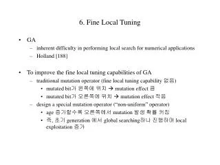
6. Fine Local Tuning. GA inherent difficulty in performing local search for numerical applications Holland [188] To improve the fine local tuning capabilities of GA traditional mutation operator (fine local tuning capability 없음) mutated bit 가 왼쪽에 위치 mutation effect 큼

E N D
6. Fine Local Tuning • GA • inherent difficulty in performing local search for numerical applications • Holland [188] • To improve the fine local tuning capabilities of GA • traditional mutation operator (fine local tuning capability 없음) • mutated bit가 왼쪽에 위치 mutation effect 큼 • mutated bit가 오른쪽에 위치 mutation effect 작음 • design a special mutation operator (“non-uniform” operator) • age 증가할수록 오른쪽에서 mutation 발생 확률 커짐 • 즉, 초기 generation 에서 global searching하나 진행하며 local exploitation 증가
6.1 The Test Cases • Optimal control problems • very difficult to design and implement • dynamic programming 기법 • widely used • suffering from what is called “the curse of dimensionality” • This Chapter • modifications of GA • FP representation • non-uniform operators • 비교 목적 • GAMS (Student Version of General Algebraic Modeling System with MINOS optimizer) 결과와 비교 • 3가지 optimal control problems 사용
6.1 The Test Cases • linear-quadratic problem • min(q xN2 + k=0, N-1 (s xk2 + ruk2)) subject to xk+1 = a xk+ b uk, k=0,1,….N-1 • analytical solution • J* = K0x02 • 10 test cases (Table 6.1) (2) the harvest problem • max k=0, N-1 (uk)1/2 subject to xk+1 = a xk– uk and one equality condition x0 = xN • analytical solution (3) The push-cart problem • maximize x1(N) – (1/2N)k=0, N-1 (uk)2 • analytical solution
6.2 The Evolution Program for Numerical Optimization • The Evolution Program (EP) • FP representation • new (specialized) genetic operators • The Representation • chromosome vector에서 각 variable이 한 개 element (FP 값) • domain 내에 들도록 초기화 & operation 결과가 domain 벗어나지 않도록 operator 설계 • precision은 machine 에만 dependent (binary 경우는 vector length와 직접 관련 high precision 위해서는 매우 긴 vector 필요 intensive computation) • 매우 큰 domain (또는 unknown domain) 표현 가능 • nontrivial constraint 다루기 위한 operator 설계 용이 (problem space와 representation space 유사)
6.2 The Evolution Program for Numerical Optimization • The Specialized Operators • Mutation group • uniform mutation • xit = <v1,…,vn> xit+1 = <v1,.., v’k,…,vn> • v’k is a random value from the domain • each element vkhaving exactly equal chance of mutation • non-uniform mutation • fine local tuning capability • svt = <v1,…,vm> svt+1 = <v1,.., v’k,…,vm>where • v’k= vk + (t,uk-vk) if a random digit is 0 vk - (t, vk -lk) if a random digit is 1 • the probability of (t,y) being close to 0 increases as t increases • property of searching the space uniformly initially (when t is small) • and very locally at later stages (when t is large) • Figure 6.1 • (t,y) 수식
6.2 The Evolution Program for Numerical Optimization • The Specialized Operators • Crossover group • simple crossover • defined in the usual way • but only permissible point s between v’s • arithmetic crossover • linear combination of two vectors • svt+1 =aswt + (1-a)svt • swt+1 =asvt + (1-a)swt • a 에따라 , a가 constant 이면 uniform arithmetic crossover age에 따르면 non-uniform arithmetic crossover • 전체 vector에 적용 또는 선택된 요소에만 적용
6.3 Experiments and Results • Experiments • optimal control problems에 대한 EP 결과 제시 • pop-size=70, 40,000 generations • 3 random runs and report the best result (run 간의 차이 무시할 정도) • Table 6.2: linear-quadratic problem • Table 6.3: harvest problem • Table 6.4: push-cart problem
6.4 Evolution Program and Other Methods • 비교 • exact solution (by analytical formula) • EP 결과 • GAMS 결과 (1) Linear –quadratic problem • Table 6.5 • GAMS는이러한 유형의 문제에 적합한 search method 사용 GAMS에게는 쉬운 문제 • EP is comparable to GAMS (2) The harvest problem • Table 6.6 • GAMS • 답과 큰 오차, N>4 동작 못함 • sensitive to non-convexity of the problem and to the number of variables • EP • good results (less than 0.001 % error)
6.4 Evolution Program and Other Methods (3) The push-cart problem • Table 6.7 • GAMS과 EP 모두 만족할 만한 결과 • 계산 효율 (variable 수에 따른) • dynamic programming: curse of dimensionality (exponential) • GAMS: worse than linear • EP: GAMS 보다 느리나 linear (Figure 6.2) • The significance of non-uniform mutation • Table 6.9 comparing ‘with non-uniform’ and ‘without non-uniform’ • non-uniform outperforms the ‘without non-uniform’
6.5 Conclusions • Non-uniform mutation • improving the fine local tuning capabilities of GA • successful results on 3 optimal control problems • reasonable computation time (CRAY Y-MP 수 분, DEC-3100 15분) • EP program 특징 • optimization function need not be continuous • user can monitor the ‘state of the search’ during the run time • linear computation time • Other methods for enhancing fine local tuning capabilities • Delta coding algorithm • Dynamic parameter encoding • ARGOT strategy • …..