Download
1 / 15
150 likes | 285 Vues
CHAPTER 11 Hierarchical Clustering. Tables, Figures, and Equations. From: McCune, B. & J. B. Grace. 2002. Analysis of Ecological Communities . MjM Software Design, Gleneden Beach, Oregon http://www.pcord.com. How it works

E N D
CHAPTER 11 Hierarchical Clustering Tables, Figures, and Equations From: McCune, B. & J. B. Grace. 2002. Analysis of Ecological Communities.MjM Software Design, Gleneden Beach, Oregon http://www.pcord.com
How it works • A dissimilarity matrix of order nn (n = number of entities) is calculated and each of the elements is squared. The algorithm then performs n-1 loops (clustering cycles) in which the following steps are done: • 1. The smallest element (dpq2) in the dissimilarity matrix is sought (the groups associated with this element are Spand Sq). • The objective function En (the amount of information lost by linking up to cycle n; see preceding chapter) is incremented according to the rule • 3. Group Sp is replaced by SpÈSq by recalculating the dissimilarity between the new group and all the other groups (practically this means replacing the pth row and column by new dissimilarities). • 4. Group Sq is rendered inactive and its elements assigned to group Sp. • After joining all items, the procedure is complete.
Table 11.1. Summary of combinatorial coefficients used in the basic combinatorial equation. • np = number of elements in Sp • nq= number of elements in Sq • nr= number of elements in Sr = SpÈSq • ni= number of elements in Si i = 1, n except i¹p and i¹q
Table 11.2. Summary of properties of linkage methods and distance measures.
The basic combinatorial equation is: where values of ap, aq, b, and g determine the type of sorting strategy (Table 11.1).
Combinatorial or noncombinatorial • Compatible or incompatible • Space-conserving or space-distorting
Table 11.3. Data matrix Table 11.4. Squared Euclidean distance matrix
Cluster step 1: Combine group 2 (plot 2) into group 1 (plot 1) at level E = 0.5. This fusion produces the least possible increase in Wishart’s objective function (below).
Obtain the coefficients for this equation by applying the formulas for Ward’s method from Table 11.1: So • Table 11.5. Revised distance matrix after the first fusion.
Figure 11.1. Agglomerative cluster analysis of four plots using Ward’s method and Euclidean distance. The data matrix is given in Table 11.3. Figure 11.2. Agglomerative cluster analysis of four plots using Ward’s method and Sørensen distance. The data are the same as for Figure 11.1.
Flexible beta (ap + aq + b = 1; ap = aq; b < 1; g = 0)
Figure 11.4. Example of effect of linkage method on dendrogram structure. Note how strongly the degree of chaining depends on the linkage method.