Comp. Genomics
Comp. Genomics. Recitation 6 14/11/06 ML and EM. Outline. Maximum likelihood estimation HMM Example EM Baum-Welch algorithm. Maximum likelihood. One of the methods for parameter estimation Likelihood: L=P(Data|Parameters) Simple example: Simple coin with P(head)=p 10 coin tosses

Comp. Genomics
E N D
Presentation Transcript
Comp. Genomics Recitation 6 14/11/06 ML and EM
Outline • Maximum likelihood estimation • HMM Example • EM • Baum-Welch algorithm
Maximum likelihood • One of the methods for parameter estimation • Likelihood: L=P(Data|Parameters) • Simple example: • Simple coin with P(head)=p • 10 coin tosses • 6 heads, 4 tails • L=P(Data|Params)=(106)p6 (1-p)4
Maximum likelihood • We want to find p that maximizes L=(106)p6 (1-p)4 • Infi 1, Remember? • Log is a monotonically increasing function, we can optimize logL=log[(106)p6 (1-p)4]= log(106)+6logp+4log(1-p)] • Deriving by p we get: 6/p-4/(1-p)=0 • Estimate for p:0.6 (Makes sense?)
ML in Profile HMMs • Emission probabilities • Mi a • Ii a • Transition Probabilities • Mi Mi+1 • Mi Di+1 • Mi Ii • Ii Mi+1 • Ii Ii • Di Di+1 • Di Mi+1 • Di Ii http://www.cs.huji.ac.il/~cbio/handouts/Class6.ppt
Parameter Estimation for HMMs Input: X1,…,Xn independent training sequences Goal: estimation of = (A,E) (model parameters) Note: P(X1,…,Xn | ) = i=1…nP(Xi | )(indep.) l(x1,…,xn | )= log P(X1,…,Xn | ) = i=1…nlog P(Xi | ) Case 1 - Estimation When State Sequence is Known: Akl = #(occurred kl transitions) Ek(b) = #(emissions of symbol b that occurred in state k) Max. Likelihood Estimators: • akl = Akl / l’Akl’ • ek(b) = Ek(b)/ b’Ek(b’) small sample, or prior knowledge correction: A’kl = Akl + rkl E’k(b) = Ek(b) + rk(b)
Example • Suppose we are given the aligned sequences **---* AG---C A-AT-C AG-AA- --AAACAG---C • Suppose also that the “match” positions are marked... http://www.cs.huji.ac.il/~cbio/handouts/Class6.ppt
**---* AG---C A-AT-C AG-AA- --AAACAG---C Calculating A, E count transitions and emissions: transitions emissions http://www.cs.huji.ac.il/~cbio/handouts/Class6.ppt
**---* AG---C A-AT-C AG-AA- --AAACAG---C Calculating A, E count transitions and emissions: transitions emissions http://www.cs.huji.ac.il/~cbio/handouts/Class6.ppt
Estimating Maximum Likelihood probabilities using Fractions emissions http://www.cs.huji.ac.il/~cbio/handouts/Class6.ppt
Estimating ML probabilities (contd) transitions http://www.cs.huji.ac.il/~cbio/handouts/Class6.ppt
EM - Mixture example • Assume we are given heights of 100 individuals (men/women): y1…y100 • We know that: • The men’s heights are normally distributed with (μm,σm) • The women’s heights are normally distributed with (μw,σw) • If we knew the genders – estimation is “easy” (How?) • What we don’t know the genders in our data! • X1…,X100are unknown • P(w),P(m) are unknown
Mixture example • Our goal: estimate the parameters (μm,σm), (μn,σn), p(m) • A classic “estimation with missing data” • (In an HMM: we know the emmissions, but not the states!) • Expectation-Maximization (EM): • Compute the “expected” gender for every sample height • Estimate the parameters using ML • Iterate
EM • Widely used in machine learning • Using ML for parameter estimation at every iteration promises that the likelihood will consistently improve • Eventually we’ll reach a local minima • A good starting point is important
Mixture example • If we have a mixture of M gaussians, each with a probability αi and density θi=(μm,σm) • Likelihood the observations (X): • The “incomplete-data” log-likelihood of the sample x1,…,xN: • Difficult to estimate directly…
Mixture example • Now we introduce y1,…,y100: hidden variables telling us what Gaussian every sample came from • If we knew y, the likelihood would be: • Of course, we do not know the ys… • We’ll do EM, starting from θg=(α1g ,..,αMg, μ1g,..,μMg,σ1g,.., σMg)
Estimation • Given θg, we can estimate the ys! • We want to find: • The expectation is over the states of y • Bayes rule: P(X|Y)=P(Y|X)P(X)/P(Y):
Estimation • We write down the Q: • Daunting?
Estimation • Simplifying: • Now the Q becomes:
Maximization • Now we want to find parameter estimates, such that: • Infi 2, remember? • To impose the constraint Sum{αi}=1, we introduce Lagrange multiplier λ: • After summing both sides over l:
Maximization • Estimating μig+1,σig+1 is more difficult • Out of scope here • What turns out is actually quite straightforward:
What you need to know about EM: • When: If we want to estimate model parameters, and some of the data is “missing” • Why: Maximizing likelihood directly is very difficult • How: • Initial guess of the parameters • Finding a proper term for Q(θg, θg+1) • Deriving and finding ML estimators
EM estimation in HMMs Input: X1,…,Xn independent training sequences Baum-Welch alg. (1972): • Expectation: • compute expected # of kl state transitions: P(i=k, i+1=l | X, ) = [1/P(x)]·fk(i)·akl·el(xi+1)·bl(i+1) Akl= j[1/P(Xj)] · i fkj(i) · akl ·el(xji+1) · blj(i+1) • compute expected # of symbol b appearances in state k Ek(b) = j[1/P(Xj)] · {i|xji=b} fkj(i) · bkj(i) (ex.) • Maximization: • re-compute new parameters from A, E using max. likelihood. repeat (1)+(2) until improvement