Gene Finding Techniques with HMMs and Phylogenetic Models in Genomics
This document explores advanced gene-finding methodologies utilizing Hidden Markov Models (HMMs) and phylogenetic approaches. It covers the limitations of traditional HMMs in detecting eukaryotic genes, the need for generalized HMMs, and the integration of phylogenetic information to improve model accuracy. Key frameworks discussed include N-SCAN and SGP2, which leverage multiple genomic sequences and conserved regions to enhance gene prediction. The outline details Markov sequence models, exon-intron dynamics, and the significance of length distributions in gene structure.

Gene Finding Techniques with HMMs and Phylogenetic Models in Genomics
E N D
Presentation Transcript
Comp. Genomics Recitation 9 11/3/06 Gene finding using HMMs & Conservation
Outline • Gene finding using HMMs • Adding trees to HMMs • phyloHMM • N-SCAN • BLAST+ Gene Finding • SGP2 • Examples
Markov Sequence Models • Key: distinguish coding/non-coding statistics • Popular models: • 6-mers (5th order Markov Model) • Homogeneous/non-homogeneous (reading frame specific) • Not sensitive enough for eukaryote genes: exons too short, poor detection of splice junctions
1-p exon intron q p 1-q Length Distribution • Simple HMMs can only encode genometric length distributions • The length of each exon (intron) :
Exon Length Distribution • The length distribution of introns is ≈ geometric • For exons, it isn’t: also affected by splicing itself: • Too short (under 50bps): the spliceosomes have no room • Too long (over 300bps): ends have problems finding each other. • But as usual there are exceptions. • A different model for exons is needed • A different model is needed for exons.
Generalized HMM(Burge & Karlin, J. Mol. Bio. 97 268 78-94) • Instead of a single char, each state omits a sequence with some length distribution
Generalized HMM(Burge & Karlin, J. Mol. Bio. 97 268 78-94) • Overview: • Hidden Markov states q1,…qn • State qihas output length distribution fi • Output of each state can have a separate probabilistic model (weight matrix model, HMM…) • Initial state probability distribution • State transition probabilities Tij
GenScan Model Burge & Karlin JMB 97
GenScan model • states = functional units on a gene • The allowed transitions ensure the order is biologically consistent. • As an intron may cut a codon, one must keep track of the reading frame, hence the three I phases: • phase I0: between codons • phase I1:: introns that start after 1st base • phase I2 : introns that start after 2nd base
Phylogenetic HMMs • Due to Siepel and Haussler • A simple gene-finding HMM looks at a single Markov process: • Along the sequence: each position is dependent on the previous position • If we incorporate sequences from multiple organisms, we can look at another process: • Along the tree: each position is dependent on its ancestor
Phylogenetic HMMs • A simple HMM can be thought of as a machine that generates a sequence • Every state omits a single character • Multinomial distribution at every state • A phyloHMM generates an MSA • Every state omits a single MSA column • Phylogenetic model at every state
Phylogenetic models in phyloHMM • Defines a stochastic process of substitution • Every position is independent • The following process occurs: • A character is assigned to the root • The character substitution occur based of some substitution matrix and based on the branch lengths • The characters at the leaves of the tree correspond to the MSA column
Phylogenetic models in phyloHMM • Different models for different states: • Different substitution rates • E.g., in exons, we’ll see less substitutions • Different patterns of substitutions • E.g., third position bias in coding sequences • Different tree topologies • E.g., following recombination
Formally • S – set of states • Ψ – phylogenetic models (instead of E in a standard HMM) • A – state transitions • b – initial probabilities
Formally • Q – substitution rate matrix (e.g., derived from PAM) • Π – background frequencies • τ – the phylogenetic tree • β – branch lengths
Formally • - Probability of a column Xi being omitted by the model ψi • Can be computed efficiently by Felsenstein’s “pruning algorithm” (recitation 6) • Joint probability of a path in the HMM and and alignment X • Viterbi, forward-backward etc. – as usual
Simple phylo-gene-finder • If the parameters are known – Viterbi can be used to find the most probably path – segmentation into coding regions Non-coding 3rd position
Phylo-gene-finder is a good idea • Use of phylogeny is important: • Imposes structure on the substitutions • Weights different pairs differently based on the evolutionary distance
N-SCAN • Another phylogeny-HMM-gene-finder • A GHHM that emits MSA columns • Annotates one sequence at a time: the target sequence • Distinguishes between a target sequence – T and other informative sequences (Is) that may contain gaps • States correspond to sequence types in the target sequence
N-SCAN • Bayesian network instead of a simple evolutionary model • Accounts for: • 5’ UTRs • Conserved non-coding • Highly conserved • No “coding” features
SGP-2 • Drawback of the described approaches: require meaningful alignment • Impossible if one of the genomes is not yet finished • An alignment is not necessary “correct”
SGP-2 • A framework working on two genomes • Idea: • Use BLAST to identify which positions are more/less conserved • Feed the BLAST scores into the gene-finding HMM • The BLAST results serve to modify the scores of the exons.
Summary • Different approaches for gene finding • Adding phylogeny generally helps • But • What about genes/exons which are specific to humans • Ape genomes are not (almost) available and too similar • Phylogenetic help almost essential in more difficult problems • Motif finding (promoter analysis) • Ultraconserved regions with no evident function