Download

1 / 126
1.36k likes | 1.94k Vues
Chapter 5 VISCOUS FLOW: PIPES AND CHANNELS. In Chapter 3 the fluid was considered frictionless, or in some cases losses were assumed or computed without probing into their underlying causes. This chapter deals with real fluids, i.e., situations in which irreversibilities are important.

E N D
In Chapter 3 the fluid was considered frictionless, or in some cases losses were assumed or computed without probing into their underlying causes. • This chapter deals with real fluids, i.e., situations in which irreversibilities are important. • Viscosity is the fluid property that causes shear stresses in a moving fluid; it is also one means by which irreversibilities or losses are developed. In turbulent flows random fluid motions, superposed on the average, create apparent shear stresses that are more important than those due to viscous shear. • This chapter: • concept of the Reynolds number developed; • characteristics that distinguish laminar from turbulent flow are presented, and the categorization of flows into internal versus external is established; • concentrates on internal-flow cases; • steady, laminar, incompressible flows are first developed, since the losses can be computed analytically.
5.1 LAMINAR AND TURBULENT FLOWS; INTERNAL AND EXTERNAL FLOWS • Laminar flow is defined as flow in which the fluid moves in layers, or laminas, one layer gliding smoothly over an adjacent layer with only a molecular interchange of momentum. • Any tendencies toward instability and turbulence are damped out by viscous shear forces that resist relative motion of adjacent fluid layers. • Turbulent flow has very erratic motion of fluid particles, with a violent transverse interchange of momentum. The Reynolds Number
The nature of the flow, i.e., whether laminar or turbulent, and its relative position along a scale indicating the relative importance of turbulent to laminar tendencies are indicated by the Reynolds number. • Two flow cases are said to be dynamically similar when • They are geometrically similar, i.e., corresponding linear dimensions have a constant ratio. • The corresponding streamlines are geometrically similar, or pressures at corresponding points have a constant ratio.
In considering two geometrically similar flow situations, Reynolds deduced that they would be dynamically similar if the general differential equations describing their flow were identical. • By changing the units of mass, length, and time in one set of equations and determining the condition that must be satisfied to make them identical to the original equations, Reynolds found that the dimensionless group ulρ/μ must be the same for both cases. • The quantity u is a characteristic velocity, l a characteristic length, ρ the mass density, and μ the viscosity. • This group, or parameter, is now called the Reynolds number R, (5.1.1)
To determine the significance of the dimensionless group, Reynolds conducted his experiments on flow of water through glass tubes (Fig. 5.1). • A glass tube was mounted horizontally with one end in a tank and a valve on the opposite end. A smooth bellmouth entrance was attached to the upstream end, with a dye jet so arranged that a fine stream of dye could be ejected at any point in front of the bellmouth. Reynolds took the average velocity V as characteristic velocity and the diameter of tube D as characteristic length, so that R = VDρ/μ. Figure 5.1 Reynolds apparatus
For small flows the dye stream moved as a straight line through the tube, showing that the flow was laminar. As the flow rate increased, the Reynolds number increased, since D, ρ, μ, were constant and V was directly proportional to the rate of flow. • With increasing discharge a condition was reached at which the dye stream wavered and then suddenly broke up and was diffused throughout the tube. The flow had changed to turbulent flow with its violent interchange of momentum that had completely disrupted the orderly movement of laminar flow. • By careful manipulation Reynolds was able to obtain a value R = 12000 before turbulence set in. A later investigator, using Reynolds' original equipment, obtained a value of 40 000 by allowing the water to stand in the tank for several days before the experiment and by taking precautions to avoid vibrations of the water or equipment. • These numbers, referred to as the Reynolds upper critical numbers, have no practical significance in that the ordinary pipe installation has irregularities that cause turbulent flow at a much smaller value of the Reynolds number.
Starting with turbulent flow in the glass tube, Reynolds found that it always becomes laminar when the velocity is reduced to make R less than 2000. This is the Reynolds lower critical number for pipe flow and is of practical importance. • With the usual piping installation, the flow will change from laminar to turbulent in the range of Reynolds numbers from 2000 to 4000. For the purpose of this treatment it is assumed that the change occurs at R = 2000. • In laminar flow the losses are directly proportional to the average velocity, while in turbulent flow the losses are proportional to the velocity to a power varying from 1.7 to 2.0. • There are many Reynolds numbers in use today in addition to the one for straight round tubes. For example, the motion of a sphere through a fluid can be characterized by UDρ/μ, in which U is the velocity of sphere, D is the diameter of sphere, and ρ and μ are the fluid density and viscosity.
The nature of a given flow of an incompressible fluid is characterized by its Reynolds number. • For large values of R one or all of the terms in the numerator are large compared with the denominator. This implies a large expanse of fluid, high velocity, great density, extremely small viscosity, or combinations of these extremes. • The numerator terms are related to inertial forces, or to forces set up by acceleration or deceleration of the fluid; the denominator term is the cause of viscous shear forces the Reynolds number parameter can also be considered as a ratio of inertial to viscous forces. • A large R indicates a highly turbulent flow with losses proportional to the square of the velocity. The turbulence may be fine-scale, composed of a great many small eddies that rapidly convert mechanical energy into irreversibilities through viscous action; or it may be large-scale, like the huge vortices and swirls in a river or gusts in the atmosphere. The large eddies generate smaller eddies, which in turn create fine-scale turbulence.
Turbulent flow may be thought of as a smooth, possibly uniform flow, with a secondary flow superposed on it. In general, the intensity of turbulence increases as the Reynolds number increases. • For intermediate values of R both viscous and inertial effects are important, and changes in viscosity change the velocity distribution and the resistance to flow. • For the same R, two geometrically similar closed-conduit systems (one, say, twice the size of the other) will have the same ratio of losses to velocity head. • The Reynolds number provides a means of using experimental results with one fluid to predict results in a similar case with another fluid.
Internal and External Flows • Another method of categorizing flows is by examining the extent of the flow field. • Internal flow involves flow in a bounded region, as the name implies. • External flow involves fluid in an unbounded region in which the focus of attention is on the flow pattern over a body immersed in the fluid. • The motion of a real fluid is influenced significantly by the presence of the boundary. • Fluid particles at the wall remain at rest in contact with the wall. In the flow field a strong velocity gradient exists in the vicinity of the wall, a region referred to as the boundary layer. • A retarding shear force is applied to the fluid at the wall, the boundary layer being a region of significant shear stresses.
This chapter deals with flows constrained by walls in which the boundary effect is likely to extend through the entire flow. • The boundary influence is easily visualized at the entrance to a pipe from a reservoir (Fig. 5.2). Figure 5.2 Entrance zone of pipeline.
At section A - A, near a well-rounded entrance, the velocity profile is almost uniform over the cross section. The action of the wall shearing stress is to slow down the fluid near the wall. As a consequence of continuity, the velocity must increase in the central region. Beyond a transitional length L' the velocity profile is fixed since the boundary influence has extended to the pipe centerline. • The transition length is a function of the Reynolds number; for laminar flow Langhaar developed the theoretical formula (5.1.2) • In turbulent flow the boundary layer grows more rapidly and the transition length is considerably shorter than given by Eq. (5.1.2). • In external flows, with an object in an unbounded fluid, the frictional effects are confined to the boundary layer next to the body (examples: golf ball in flight, an airfoil, and a boat). • The fully developed velocity profile is unlikely to exist in external flows. Typically interest is focused on drag forces on the object or the lift characteristics developed on the body by the particular flow pattern.
5.2 NAVIER-STOKES EQUATIONS • The equations of motion for a real fluid can be developed from consideration of the forces acting on a small element of the fluid, including the shear stresses generated by fluid motion and viscosity. • The derivation of these equations, called the Navier-Stokes equations, is beyond the scope of this treatment. They are listed, however, for the sake of completeness, and many of the developments of this chapter could be made directly from them. • First, Newton's law of viscosity for one-dimensional laminar flow can be generalized to three-dimensional flow (Stokes' law of viscosity) (5.2.1) • The first subscript of the shear stress is the normal direction to the face over which the stress component is acting. The second subscript is the direction of the stress component.
In Chap. 3, in developing the Euler and energy equations, z was taken as the vertical coordinate, so that z was a measure of potential energy per unit weight. • In dealing with problems it is convenient to allow the x, y, z system of right-angular coordinates to take on any arbitrary orientation. • Since gravity, the only body force considered, always acts vertically downward, h is taken as a coordinate which is positive vertically upward; then ∂h/∂x is the cosine of the angle between the x axis and the h axis, and similarly for the y and z axes.
(5.2.2) (5.2.3) (5.2.4) • When the Navier-Stokes equations are limited to incompressible fluids, they become • in which v is the kinematic viscosity, assumed to be constant, d/dt is differentiation with respect to the motion • and • For a nonviscous fluid, the Navier-Stokes equations reduce to the Euler equations of motion in three dimensions, (8.2.3) to (8.2.5).
For one-dimensional flow of a real fluid in the l direction (Fig. 5.3) with h vertically upward and y normal to l (v = 0, w = 0, ∂u/∂l = 0), the Navier-Stokes equations reduce to (5.2.5) (5.2.6) • For steady flow (5.2.7) • Since u is a function of y only, τ = μdu/dy for one-dimensional flow, and (5.2.8)
Figure 5.3 Flow between inclined parallel plates with the upper plate in motion
5.3 LAMINAR, INCOMPRESSIBLE, STEADY FLOW BETWEEN PARALLEL PLATES • The general case of steady flow between parallel inclined plates is first developed for laminar flow, with the upper plate having a constant velocity U (Fig. 5.3). • Flow between fixed plates is a special case obtained by setting U = 0. In Fig. 5.3 the upper plate moves parallel to the flow direction, and there is a pressure variation in the l direction. The flow is analyzed by taking a thin lamina of unit width as a free body. • In steady flow the lamina moves at constant velocity u. The equation of motion yields • Dividing through by the volume of the element, using sin Θ = -∂h/∂l, and simplifying yields
(5.3.1) • Integrating Eq. (5.3.1) with respect to y yields • Integrating again with respect to y leads to • in which A and B are constants of integration. To evaluate them, take y = 0, u = 0 and y = a, u = U and obtain • Eliminating A and B results in (5.3.2)
For horizontal plates, h = C; for no gradient due to pressure or elevation, i.e., hydrostatic pressure distribution, p + γh =C and the velocity has a straight-line distribution. • For fixed plates, U = 0, and the velocity distribution is parabolic. • The discharge past a fixed cross section is obtained by integration of Eq. (5.3.2) with respect to y: (5.3.3) • In general, the maximum velocity is not at the midplane.
Example 5.1 • In Fig. 5.4 one plate moves relative to the other as shown; μ = 0.08 Pa · s; ρ = 850 kg/m3. Determine the velocity distribution, the discharge, and the shear stress exerted on the upper plate. Solution • At the upper point • And at the lower point • To the same datum. Hence,
From the figure, a = 0.006 m, U = -1 m/s; and from Eq. (5.3.2) • The maximum velocity occurs were du/dy = 0, or y = 0.00079 m, and it is umax = 0.0236 m/s. The discharge per meter of width is • Which is upward. To find the shear stress on the upper plate, • And • This is the fluid shear at the upper plate; hence, the shear force on the plate is 31.44 Pa resisting the motion of the plate.
Losses in Laminar Flow • Expressions for irreversibilities are developed for one-dimensional, incompressible, steady, laminar flow. For steady flow in a tube, between parallel plates, or in a film flow at constant depth, the kinetic energy does not change and the reduction in p + γh represents the work done on the fluid per unit volume. The work done is converted into irreversibilities by the action of viscous shear. The losses in length L are QΔ(p + γh) per unit time. • If u is a function of y, the transverse direction, and the change in p + γh is a function of distance x in the direction of flow, total derivatives may be used throughout the development. First, from Eq. (5.3.1) (5.3.4) • With reference to Fig. 5.5, a particle of fluid of rectangular shape of unit width has its center at (x, y), where the shear is τ, the pressure p, the velocity u, and the elevation h. It moves in the x direction.
Figure 5.5Work done and loss of potential energy for a fluid particle in one-dimensional flow
In unit time it has work done on it by the surface boundaries as shown, and it gives up potential energy γδx δy u sin Θ. As there is no change in kinetic energy of the particle, the net work done and the loss of potential energy represent the losses per unit time due to irreversibilities. • Collecting the terms from Fig. 5.5, dividing through by the volume δx δy, and taking the limit as δx δy goes to zero yields (5.3.5) • By combining with Eq. (5.3.4) (5.3.6)
Integrating this expression over a length L between two parallel plates, with Eq. (5.3.2) for U = 0, gives • Substituting for Q from Eq. (5.3.3) for U = 0 yields • in which Δ(p + γh) is the drop in p + γh in the length L. The expression for power input per unit volume [Eq. (5.3.6)] is also applicable to laminar flow in a tube. The irreversibilities are greatest when du/dy is greatest. • The distribution of shear stress, velocity, and losses per unit volume is shown in Fig. 5.6 for a round tube.
Figure 5.6 Distribution of velocity, shear, and losses per unit volume for a round tube
Example 5.2 • A conveyor-belt device, illustrated in Fig. 5.7, is mounted on a ship and used to pick up undesirable surface contaminants, e.g., oil, from the surface of the sea. Assume the oil film to be thick enough for the supply to be unlimited with respect to the operation of the device. • Assume the belt to operate at a steady velocity U and to be long enough for a uniform flow depth to exist. • Determine the rate at which oil can be carried up the belt per unit width, in terms of Θ, U, and the oil properties μ and γ. Solution • A thin lamina of unit width that moves at velocity u is shown in Fig. 5.7. With the free surface as shown on the belt, and for steady flow at constant depth, the end-pressure effects on the lamina cancel. • The equation of motion applied to the element yields
When the shear stress at the surface is recognized as zero, integration yields • This equation can be combined with Newton’s law of viscosity, τ = -μdu/dy, to give • or • The flow rate per unit width up the belt can be determine by integration: • This expression shows the flow rate to vary with a. However, a is still a dependent variable that is not uniquely defined by the above equations. The actual depth of flow on the belt is controlled by the end conditions.
The depth for maximum flow rate can be obtained by setting the derivative dq/da to zero and solving for the particular a • To attach some physical significance to this particular depth, the influence of alternative crest depths may be considered. If the crest depth A, Fig. 5.7, is such that a occurs on the belt, then the maximum flow for that belt velocity and slope will be achieved. If A is physically controlled at a depth greater than a, more flow will temporarily be supplied by the belt than can get away at the crest. • That will cause the belt depth to increase and the flow to decrease correspondingly, until either an equilibrium condition is realized or A is lowered. Alternatively, if A < a, flow off the belt will be less than the maximum flow up the belt at depth a and the crest depth will increase to a.
At all times it is assumed that an unlimited supply is available at the bottom. By this reasoning it is seen that a is the only physical flow depth that can exist on the belt if the crest depth is free to seek its own level. A similar reasoning at the base leads to the same conclusion. • The discharge, as a function of fluid properties and U and Θ, is given by • or
5.4 LAMINAR FLOW THROUGH CIRCULAR TUBES AND CIRCULAR ANNULI • For steady, incompressible, laminar flow through a circular tube or an annulus, a cylindrical infinitesimal sleeve (Fig. 5.8) is taken as a free body. The equation of motion is applied in the l direction, with acceleration equal to zero. • From the figure, • Replacing sin Θ by –dh/dl and dividing by the volume of the free body, 2πrδrδl, gives (5.4.1)
Figure 5.8 Free-body diagram of cylindrical sleeve element for laminar flow in an inclined circular tube
Since d(p + γh)/dl is not a function of r, the equation can be multiplied by rδr and integrated with respect to r, yielding (5.4.2) • In which A is the constant of integration. For a circular tube this equation must be satisfied when r = 0; hence, A = 0 for this case. Substituting • Note that the minus sign is required to obtain the sigh of the τ term in Fig. 5.8 (u is considered to decrease with r; hence, du/dr is negative) • Another integration gives (5.4.3)
For the annual case, to evaluate A and B, u = 0 when r = b, the inner tube radius, and u = 0 when r = a (Fig. 5.9). When A and B are eliminated, (5.4.4) • And for discharge through an annulus (Fig. 5.9), (5.4.5)
Circular Tube; Hagen-Poiseuille Equation • For the circular tube, A = 0 in Eq. (5.4.3) and u = 0 for r = a, (5.4.6) • The maximum velocity umax is given for r = 0 as (5.4.7) • Since the velocity distribution is a paraboloid of revolution (Fig. 5.6), its volume is one-half that of its circumscribing cylinder; therefore, the average velocity is one-half of the maximum velocity, (5.4.8) • The discharge Q is equal to Vπa2, (5.4.9)
The discharge can also be obtained by integration of the velocity u over the area, i.e., • For a horizontal tube, h = const; writing the pressure drop Δp in the length L gives • And substituting diameter D leads to (5.4.10a) • In terms of average velocity, (5.4.10b)
Equation (5.4.10a) can then be solved for pressure drop, which represents losses per unit volume, (5.4.11) • The losses are seen to vary directly as the viscosity, the length, and the discharge and to vary inversely as the fourth power of the diameter. It should be noted that tube roughness does not enter into the equations. • Equation (5.4.10a) is known as the Hagen-Poiseuille equation. • The kinetic-energy correction factor α [Eq. (3.10.2)] can be determined for laminar flow in a tube by use of Eqs. (5.4.6) and (5.4.7) (5.4.12) • Substituting into the expression for α gives (5.4.13) • There is twice as much energy in the flow as in uniform flow at the same average velocity.
Example 5.3 • Determine the direction of flow through the tube shown in Fig. 5.10, in which γ = 8000 N/m3 and μ = 0.04 Pa · s. Find the quantity flowing in liters per second and calculate the Reynolds number for the flow. Solution • At section 1: • and at section 2: • if the elevation datum is taken through section 2. The flow is from 2 to 1, since the energy is greater at 2 (kinetic energy must be the same at each section) than at 1. To determine the quantity flowing, the expression is written • With l positive from 1 to 2.
Substituting into Eq. (5.4.9) gives • The average velocity is • And the Reynolds number is • If the Reynolds number had been above 2000, the Hagen-Poiseuille equation would no longer apply.
5.5TURBULENT SHEAR RELATION • In turbulent flow the random fluctuations of each velocity component and pressure term in Eqs. (5.2.2) make exact analysis difficult if not impossible, even with numerical methods. • It becomes more convenient to separate the quantities into mean or time-averaged values and fluctuating parts. The x component of velocity u, for example, is represented by (5.5.1) • As shown in Fig. 5.11, in which the mean value is the time-averaged quantity defined by (5.5.2)
The limit T on the integration is an averaging time period, suitable to the particular problem, that is grater than any period of the actual variations. • We note in Fig. 5.11 and from the definition that the fluctuation has a mean value of zero (5.5.3) • However, the mean square of each fluctuation is not zero (5.5.4) • The square root of this quantity, the root mean square of measured values of the fluctuations, is a measure of the intensity of the turbulence. Reynolds split each property into mean and fluctuating variables • In each case the mean value of the fluctuation is zero and the mean square is not.
Substitution of the mean and fluctuating parts of the variables into the continuity equation (3.4.9) for incompressible flow yields (5.5.5) • In the x direction the equation reduces to (5.5.6) • We note that the three terms , and have the same effect in the equation as the mean viscous-shear stress. They are actually convective-acceleration term, but since they mathematically provide a stress like effect, they are identified with Reynolds stresses. • Since in general the Reynolds stress are unknown, empirical methods based upon intuitive reasoning, dimensional analysis, or physical experiments are used to assist in analysis.
In one-dimensional flow in the x direction the turbulent stress is the most important, and linear-momentum equation can be approximated by (5.5.7) • in which (5.5.8) • is a total shear made up of laminar τl and turbulent τt components. In view of the difficulty of evaluating , Prandtl introduced the mixing-length theory, which relates the apparent shear stress to the temporal mean velocity distribution.