Simulation Based Power Estimation For Digital CMOS Technologies
Simulation Based Power Estimation For Digital CMOS Technologies Master’s Thesis Defense Jins Davis Alexander. Thesis Advisor: Dr. Vishwani D. Agrawal Thesis Committee: Dr. Victor P. Nelson and Dr. Adit Singh. Department of Electrical and Computer Engineering Auburn University, AL 36849 USA.


Simulation Based Power Estimation For Digital CMOS Technologies
E N D
Presentation Transcript
Simulation Based Power Estimation For Digital CMOS Technologies Master’s Thesis DefenseJins Davis Alexander • Thesis Advisor:Dr. Vishwani D. Agrawal • Thesis Committee:Dr. Victor P. Nelson and Dr. Adit Singh Department of Electrical and Computer Engineering Auburn University, AL 36849 USA MS Thesis Defense
Outline • Motivation and Problem Statement • Background • Contributions: • PowerSim: A Generalized Power Analysis Tool • A New Dynamic Power Analysis Algorithm • Bounded Delays and Ambiguity Intervals • Maximum Transitions • Minimum Transitions • Simulation and Power Estimation • Experimental Results and Observations • Conclusion MS Thesis Defense
Motivation • Dynamic power increases with glitch transitions, which in turn are a functions of gate delays. • Process variation can influence delays in a circuit, especially in nanoscale technologies. • Monte Carlo simulation used to address the variation is time consuming and CPU intensive. • Bounded delay models are usually considered to address process variations in logic level simulation and timing analysis (Grimes, MS Thesis, August 2008). MS Thesis Defense
Problem Statement • Given a set of vectors (random or selected functional set): • Analyze a digital circuit for various power components (dynamic – logic and glitch, short circuit, leakage, clock, flip-flop) in a nominal delay circuit. • Determine the range of dynamic power consumption for specified bounds on delay variations. MS Thesis Defense
C880: Monte Carlo vs. New Method 1000 Random Vectors, 1000 Sample Circuits MS Thesis Defense
Background • Bounded delays model delay uncertainties by assigning each gate lower and upper bounds on delay, also known as min–max delays. • The bounds can be obtained by adding specified process-related variation to the nominal gate delay for the technology. • In this model, regions of signal uncertainties are defined at the output of each gate node. MS Thesis Defense
Specifying Ambiguity Delay Intervals IV FV IV FV EA LS EA LS • EA is the earliest arrival time • LS is the latest stabilization time • IV is the initial signal value • FV is the final signal value EAsv=-∞ LSsv=∞ EAdv LSdv EAdv=-∞ LSdv=∞ EAsv LSsv MS Thesis Defense
Propagating Ambiguity Intervals through Gates The ambiguity interval (EA,LS) for a gate output is determined from the ambiguity intervals of input signals, their pre-transition and post-transition steady-state values, and the min-max gate delays. (mindel, maxdel) MS Thesis Defense
Representative Formulae • To evaluate the output of a gate, we analyze inputs i: MS Thesis Defense
Formulae… • and, where the inertial delay of the gate is bounded as (mindel, maxdel). MS Thesis Defense
Finding Number of Transitions 3 14 7 10 12 14 2 5 8 10 12 [mintran,maxtran] [0,2] 3 14 (mindel, maxdel) 6 17 1,3 EA LS EA LS [0,4] 5 17 EA LS where mintran is the minimum number of transitions and maxtran the maximum number of transitions. MS Thesis Defense
Estimating maxtran • First upper bound: We calculate the maximum transitions (Nd) that can be accommodated in the ambiguity interval given by the gate delay bounds and the (IV,FV) output values. • Second upper bound: We take the sum of the input transitions (N) as the output cannot exceed this. We modify this by : N = N – k (1) where k = 0, 1, or 2 for a 2-input gate and is determined by the ambiguity regions and (IV, FV) values of inputs. • The maximum number of transitions is lower of the two upper bounds: maxtran = min (Nd, N) (2) MS Thesis Defense
Examples of maxtran (k = 0) Nd = ∞ N = 8 maxtran=min (Nd, N) = 8 Nd = 6 N = 8 maxtran=min (Nd, N) = 6 MS Thesis Defense
Example: maxtran With Non-Zero k [n1 = 6] [n1 + n2 – k = 8 ] , where k = 2 EA LS EAsv = - ∞ LSdv = ∞ EAdv LSsv [n2 = 4] EAsv = - ∞ LSdv = ∞ EAdv LSsv [ 6 ] [ 6 + 4 – 2 = 8 ] [ 4 ] MS Thesis Defense
Estimating mintran • First lower bound (Ns): Based on steady state values, i.e., 00, 11 as no transition and 01, 10 as a single transition. • Second lower bound (Ndet): The minimum number of transitions that can occur in the output ambiguity region is the number of deterministic signal changes that occur within the ambiguity region and such that signal changes are spaced at time intervals greater than or equal to the inertial delay of the gate. • The minimum number of transitions is the higher of the two lower bounds: mintran = max (Ns, Ndet) (3) MS Thesis Defense
Example: mintran • There will always be a hazard in the output as long as (EAsv – LSdv) ≥maxdel • Thus in this case the mintran is not 0 as per the steady state condition, but is 2. EA LS EAsv = - ∞ LSsv = ∞ EAdv LSdv d EAdv = - ∞ LSdv = ∞ (mindel, maxdel) EAsv LSsv MS Thesis Defense
Multiple Ambiguity Intervals • Multiple ambiguity regions may rise in output which are separated by regions of deterministic signal states. • We arrange the (EA,LS) values in order of their temporal occurrences. • If an (LS) value occurs before an (EA) value, then a multiple ambiguity region exists. • We propagate them to the output on the condition that any two consecutive bound values are separated at least by the gate inertial delay. MS Thesis Defense
Example EA1 LS1 EA1+ d1 LS3 + d2 EA2 LS2 d1,d2 EA3 LS3 (a) EA1 LS1 EA1+ d1 EA3 + d1 EA2 LS2 d1,d2 LS2 + d2 LS3 + d2 EA3 LS3 (b) MS Thesis Defense
Simulation Methodology • maxdel, mindel = nominal delay ± Δ% • Three linear-time passes for each input vector: • First pass: zero delay simulation to determine initial and final values, IV and FV, for all signals. • Second pass: determines earliest arrival (EA) and latest stabilization (LS) from IV, FV values and bounded gate delays. • Third pass: determines upper and lower bounds, maxtran and mintran, for all gates from the above information. MS Thesis Defense
Effect of Gate Delay Distribution • Experiment conducted to see if the distribution of gate delays has an effect on power distribution. • For uniform distribution: Gate delays were randomly sampled from uniform distribution [a, b], where a = nominal delay – Δ% and b = nominal delay + Δ% This distribution has a variance σ2 = (1/12)(b – a)2 = Δ2(nom. delay)2/30,000. • For normal distribution: Gate delays were randomly sampled from a Gaussian density with mean = nom. delay, and variance σ2 as above. MS Thesis Defense
Experimental Setup • A standard gate node delay of 100 ps was taken. A wire load delay model was followed with each nominal gate delay being a function of its fan – out. • The power distribution is for 1000 random vectors with a vector period of 10000 ps. • For each vector pair 1000 sample circuits was simulated. MS Thesis Defense
UniformDistribution NormalDistribution MS Thesis Defense
Experimental Result (Maximum Power) • Monte Carlo Simulation vs. Min-Max analysis for circuit C880. 100 sample circuits with + 20 % variation were simulated for each vector pair (100 random vectors). R2 is coefficient of determination, equals 1.0 for ideal fit. MS Thesis Defense
Result…(Minimum Power) R2 is coefficient of determination, equals 1.0 for ideal fit. MS Thesis Defense
Results…(Average Power) R2 is coefficient of determination, equals 1.0 for ideal fit.
Effect of Inertial Delay • Transition Statistics for high activity gate 1407 in c2670 for a random vector pair. Histograms obtained from Monte Carlo Simulations of 100 sample circuits. mintran = 0 maxtran =1 0 maxtran = 8 mintran = 0 MS Thesis Defense
Effect of Inertial Delay… mintran = 0 mintran = 0 maxtran = 6 maxtran = 4 MS Thesis Defense
Power Estimation Result • Circuits implemented using TSMC025 2.5V CMOS library , with standard size gate delay of 10 ps and a vector period of 1000 ps. Min-Max values obtained by assuming ± 20 % variation. The simulation was run on a UNIX operating system using a Intel Duo Core processor with 2 GB RAM. MS Thesis Defense
PowerSim A gate level power analysis tool to efficiently and accurately estimate and separate the different power components. Libraries are characterized by SPICE for leakage power (all input states), node capacitance, temperature, supply voltage and other technology constraints. The tool does an event driven simulation of input vectors and estimates power from the dynamically created libraries. Provides information of the effect of different power components with respect to the circuitand technology used. Sept 3, 2008 MS Thesis Defense 29
PowerSim Results on Benchmarks Average power dissipation of ISCAS85 Benchmark circuits for 1000 random vectors, vector period 100ns, 0.25 micron CMOS technology, supply voltage 2.5 volts. Sept 3, 2008 MS Thesis Defense 30
Histogram of c880 Leakage Power Sept 3, 2008 Histogram of leakage power for circuit c880 in 90 nm technology for 1000 random vectors. MS Thesis Defense 31
Short Circuit Power Against Sizing Sept 3, 2008 The average short circuit power dissipation for 6 invertors (last inverter being used as a load) with constant size, increasing size and decreasing size. An input signal of 0 1 0 was applied to the first inverter. MS Thesis Defense 32
Conclusion • We have used bounded delay model to successfully develop a power estimation method with consideration of uncertainties in delays. • Linear time complexity in number of gates and an efficient alternative to the Monte Carlo analysis. • Future work includes considering process dependent variation in leakage as well as in node capacitances. • PowerSim is a useful gate level power analysis tool for VLSI designers. MS Thesis Defense
Thank You. MS Thesis Defense