Atmospheric Composition Sounding
Atmospheric Composition Sounding. ESA Summer School ESRIN 12 th August 2010 Lecture 1 by B.Kerridge Part 1 – Introduction

Atmospheric Composition Sounding
E N D
Presentation Transcript
Atmospheric Composition Sounding ESA Summer School ESRIN 12th August 2010 Lecture 1 by B.Kerridge Part 1 – Introduction Part 2 – mm-wave limb sounding ESA Summer School - Atmospheric Composition Sounding - B.Kerridge ESRIN, Aug’2010
Outline Aim of three lectures: overview atmospheric composition sounding from space Lecture 1 Part 1 - Introduction Scientific imperative Operational applications Evolution of models & assimilation systems Challenges imposed by physics Part 2 - mm-wave limb-sounding Principles Instrument attributes Linear retrieval diagnostics Odin SMR and Aura MLS Summary and future advances ESA Summer School - Atmospheric Composition Sounding - B.Kerridge ESRIN, Aug’2010
The atmosphere is constantly changing ESA Summer School - Atmospheric Composition Sounding - B.Kerridge ESRIN, Aug’2010 Introduction 3
ESA Living Planet Symposium - Atmospheric Composition - B.Kerridge Bergen, 27th June 2010 4
Understanding of atmospheric phenomena, including clouds and aerosol, depends upon remote-sensing observations ESA Summer School - Atmospheric Composition Sounding - B.Kerridge ESRIN, Aug’2010 Introduction 5
1. Scientific Imperative Atmospheric composition is driving climate change Primary radiative forcing by trace gases & aerosol Indirect effects through chemistry and aerosol-cloud Feedbacks via water vapour, cloud & trace gases ESA Summer School - Atmospheric Composition Sounding - B.Kerridge ESRIN, Aug’2010 Introduction 6
Scientific Imperative (contd) Remote-sensing plays a vital role to investigate processes for international assessments (IPCC,WMO) Satellites: global to regional scales Airborne / surface: finer scales; ground-truth Troposphere is challenging ESA Summer School - Atmospheric Composition Sounding - B.Kerridge ESRIN, Aug’2010 Introduction 7
Scientific objectives for sounding composition from space Processes controlling distributions of key trace gases within height-range important to climate Links to biogenic, pyrogenic and anthropogenic emissions Advances will be made in future by resolving structure on finer-scales to understand processes Requirements are stringent. ESA Summer School - Atmospheric Composition Sounding - B.Kerridge ESRIN, Aug’2010 Introduction 8
Operational Applications for Satellite Composition Data • Ozone Layer & Surface UV • satellite global observations have 30-year heritage • Composition – Climate Interaction • satellites observe trace gas profiles, aerosol & cloud which cannot be monitored adequately from surface alone • decadal, self-consistent data sets → GCOS essential climate variables (ECVs) • Pollution Monitoring & Air Quality Forecasting • satellites observe pollutants above and between surface sites ESA Living Planet Symposium - Atmospheric Composition - B.Kerridge Bergen, 27th June 2010 9
3. Evolution of models and assimilation systems Models are evolving rapidly Increased computer power enables: More complete atmospheric physics, dynamics & chemistry Integration of troposphere and stratosphere Couplings with land and ocean for climate-composition interaction Assimilation systems in development to exploit satellite data in addition to surface level observations, analogous to NWP Inverse modelling to quantify surface emissions Model resolution to increase in coming decade Processes that were sub-grid scale will be resolved (eg convection) To critically test future models, satellite observations of increased resolution will be needed. ESA Summer School - Atmospheric Composition Sounding - B.Kerridge ESRIN, Aug’2010 Introduction 10
ESA Living Planet Symposium - Atmospheric Composition - B.Kerridge Bergen, 27th June 2010 11 http://daac.gsfc.nasa.gov/fieldexp/TOGA/cls.shtml
Spectral line interference ← pressure broadening Water vapour & other continua Clouds Discriminating surface ← especially critical for aerosol Seeing through higher layers ← nb tropospheric O3 Vertical resolution in tropopause region and near-surface layer where height leverage from T profile is minimum The challenge is: to achieve significantly higher vertical resolution, horizontal resolution and spatio-temporal sampling while preserving/improving accuracy 4. Challenges imposed by physics ESA Summer School - Atmospheric Composition Sounding - B.Kerridge ESRIN, Aug’2010 Introduction 12
Part 2 – mm-wave limb-sounding Profiling mid/upper troposphere & lower stratosphere where climate sensitivity is greatest ESA Summer School - Atmospheric Composition Sounding: - B.Kerridge ESRIN, Aug’2010 mm-wave limb sounding
1) Principles of mm-wave sounding In microwave – sub-millimetre-wave region l > 100mm (0.1mm), n < 100 cm-1, f < 3THz most molecular transitions are pure rotational Rotational levels closely-spaced in energy (Dn ~1 cm-1) Collisions with N2 & O2 maintain Boltzmann population distributions of rotational levels up to the thermosphere TR → Tk – local kinetic temperature J(n,TR) → B(n,TK) – local thermodynamic equilibrium (LTE) Departure from LTE can be significant at mid-IR and shorter l’s radiative and photochemical processes can affect populations of vibrational levels (Dn ~1,000 cm-1) and electronic levels (Dn ~10,000 cm-1) in stratosphere and above have to be modelled in some cases, even if targeting low atmosphere ESA Summer School - Atmospheric Composition Sounding: - B.Kerridge ESRIN, Aug’2010 mm-wave limb sounding
Radiative Transfer Equation at Long Wavelengths (Assuming boundary emissivity =1) Planck Function If (Rayleigh-Jeans) ESA Summer School - Atmospheric Composition Sounding: - B.Kerridge ESRIN, Aug’2010 mm-wave limb sounding
Radiative Transfer Equation at Long Wavelengths continued Planck Function linearly dependent on T(z) cf IR wavelengths “Brightness Temperature” defined as: • Simplest form of atmospheric radiative transfer equation, except for • direct-sun absorption. • Applies unless surface reflectivity (nadir) or cloud scattering are non-zero • For limb geometry, boundary is “cold space” . ESA Summer School - Atmospheric Composition Sounding: - B.Kerridge ESRIN, Aug’2010 mm-wave limb sounding
Atmospheric transmittance spectra for limb-geometry(H2O, O2 & O3 only) 0 – 1000 GHz Wings of strong H2O lines control spectral curvature & penetration depth in limb-views Troposphere seen in limb-views <380GHz 12km 10km Transmittance 8km 6km Frequency (GHz) ESA Summer School - Atmospheric Composition Sounding: - B.Kerridge ESRIN, Aug’2010 mm-wave limb sounding
Wavelength Dependence of Cirrus Extinction 1mm IR sounders eg MIPAS & IASI MARSCHALS • Mm-wave affected only by scattering from large ice particles (> 80mm) • To observe smaller cirrus size components would require frequencies up to ~THz • Thin tropical tropopause cirrus, PSCs and aerosols: Re < 10 mm • These particulates transparent in mm-wave ESA Summer School - Atmospheric Composition Sounding: - B.Kerridge ESRIN, Aug’2010 mm-wave limb sounding
2) Instrument Attributes • Heterodyne (coherent) detection: • Signal from atmosphere mixed with local oscillator (LO) signal • Down-conversion to intermediate frequency (IF) band for amplification • Either upper & lower frequency bands superposed (DSB) or one band filtered out (SSB) or side-bands separated • Spectral resolution intrinsically high (bandwidth a more limiting factor) • aDoppler(1000mm) = 0.01 x aDoppler(10mm) • Lines p-broadened throughout strat. and fully-resolvable →height leverage • NEBT (K) ~ Tsys (K) / √ [ tint (s) x df (Hz) ] • AW ~ l2 ← Throughput determined by wavelength • Long wavelengths: diffraction limited optics • From polar orbit at 800km, vertical half-power beamwidth (HPBW) of 2km at tangent-point requires ~1.6m antenna at l = 1mm • For l >1mm, HPBW proportionally larger for same antenna size. ESA Summer School - Atmospheric Composition Sounding: - B.Kerridge ESRIN, Aug’2010 mm-wave limb sounding
Spectra Simulated for MLS bands at 190 GHz (R2) and 240 GHz (R3) bands H2O HNO3 HNO3 O3 O3 O3 O3 O3 O3 CO ESA Summer School - Atmospheric Composition Sounding: - B.Kerridge ESRIN, Aug’2010 mm-wave limb sounding
H2O Weighting Functions for MLS ESA Summer School - Atmospheric Composition Sounding: - B.Kerridge ESRIN, Aug’2010 mm-wave limb sounding
O3 Weighting Functions for MLS ESA Summer School - Atmospheric Composition Sounding: - B.Kerridge ESRIN, Aug’2010 mm-wave limb sounding
CO Weighting Functions for MLS ESA Summer School - Atmospheric Composition Sounding: - B.Kerridge ESRIN, Aug’2010 mm-wave limb sounding
3) Linear Retrieval Diagnostics ESA Summer School - Atmospheric Composition Sounding: - B.Kerridge ESRIN, Aug’2010 mm-wave limb sounding
Influence of antenna width & oversamplingon profile retrieval precision & resolution • Retrieval of H2O, O3, CO & HNO3 profiles simulated for idealized case: • MLS 190 & 240 GHz bands; contiguous, Df =100MHz • MLS Tsys(DSB) 1000K; scan range & duration fixed • 2km retrieval level spacing; √So(i,i) = 100% (diagonals) • Antenna: nominal HPBWs (4.2 or 3.2km) or pencil beam • Limb-view spacing: 300m or 2km • Retrieval linear diagnostics examined: • Averaging kernels, AK FWHM and √ [ Sx(i,i) / So(i,i)] ESA Summer School - Atmospheric Composition Sounding: - B.Kerridge ESRIN, Aug’2010 mm-wave limb sounding
Averaging Kernels for MLS Averaging kernels indicate: • vertical resolution of retrieval • improvement on prior knowledge • HPBW: ~4km (190 GHz) , ~3km (230GHz) • Vertical resolution <HPBW achievable for H2O and O3 • tangent-height spacing 2km • p-broadening ESA Summer School - Atmospheric Composition Sounding: - B.Kerridge ESRIN, Aug’2010 mm-wave limb sounding
Influence of antenna beam width and limb view spacing on retrieval: O3 & H2O ESD & AK FWHM R2 Antenna: HPBW: 3.2km antenna convolved not convolved 300m spacing R1 Antenna: HPBW: 4.2km not convolved antenna convolved 300m spacing ESA Summer School - Atmospheric Composition Sounding: - B.Kerridge ESRIN, Aug’2010 mm-wave limb sounding
R1 Antenna HPBW: 4.2km antenna not convolved R2 Antenna: HPBW: 3.2km antenna not convolved Influence of antenna beam width and limb view spacing on retrieval: HNO3 & CO ESD & AK FWHM ESA Summer School - Atmospheric Composition Sounding: - B.Kerridge ESRIN, Aug’2010 mm-wave limb sounding
Antenna pattern width & oversampling • Vertical resolution <HPBW achievable from spectral lineshape and oversampling • Provided radiometric sensitivity sufficiently high • Also assuming: perfect knowledge of antenna-pattern & tangent-point spacings • For real antenna and retrieval level spacing of 2km, additional benefit from reducing limb-view spacing from 2km to 300m is limited. ESA Summer School - Atmospheric Composition Sounding: - B.Kerridge ESRIN, Aug’2010 mm-wave limb sounding
Key Instrumental Uncertainties Pressure of a reference limb-view in scan & T profile can be retrieved accurately In addition to NEBT, precision & accuracy of constituent retrieval depend on knowledge of: Vertical spacings of limb-views Vertical shape of antenna pattern (for convolution of pencil beams) Critical for upper troposphere: H2O vertical gradient; clouds lower down Beam efficiency and loss BB calibration target cannot be in front of antenna Frequency-dependent responses of upper & lower side-bands Particularly for “double side-band” receivers Spectral baseline Especially structure on scales similar to atmospheric emission features ESA Summer School - Atmospheric Composition Sounding: - B.Kerridge ESRIN, Aug’2010 mm-wave limb sounding
4) Odin SMR & Aura MLS • Odin Sub-Millimetre Radiometer (SMR) • Aura Microwave Limb Sounder (MLS) • Satellite limb-emission sounders launched 2002/3 ESA Summer School - Atmospheric Composition Sounding: - B.Kerridge ESRIN, Aug’2010 mm-wave limb sounding
ODIN SMR Technical Specifications The Instrument: • Antenna size: 1.1 m • Beam size at 119/550 GHz: 9.5'/ 2.1'(126") • Main beam efficiency 90% • Pointing uncertainty <10" (rms) • Submm tuning range: 486–504, 541–581 GHz • Submm Tsys(SSB): 3300 K ← Cooling to 80K • HEMT:118.75 GHz; Tsys (SSB): 600 K • AOS b’width / res.:1100 MHz / 1 MHz • DAC b’width /res:100–800 MHz / 0.25–2 MHz The satellite:Orbit: sun-synchronous dawn-dusk, polar orbit, altitude 600 km Platform: 3-axis stabilized (reaction wheels, star sensors, gyros) Mass: 250 kg (bus 170 kg, instruments 80 kg) Size: Height 2m, width 3.8m (incl. solar panels) ESA Summer School - Atmospheric Composition Sounding: - B.Kerridge ESRIN, Aug’2010 mm-wave limb sounding
Enhanced by PSCs Descent in vortex of air low in N2O • Odin SMR sees through PSCs to observe trace gases in Antarctic ozone hole Example Single Side-Band LimbSpectra from SMR ESA Summer School - Atmospheric Composition Sounding: - B.Kerridge ESRIN, Aug’2010 mm-wave limb sounding
Odin SMR Distributions in S.Hem. Lower Strat. 19th Sept – 5th Oct 2002 • Vortex centred: • N2O low – desc. • NOylow – denit. • ClO high – act. • O3 hole Warming splits vortex Vortex reforms ClO converted back to Cl reservoirs 500K surface ~ 20km ESA Summer School - Atmospheric Composition Sounding: - B.Kerridge ESRIN, Aug’2010 mm-wave limb sounding
Aura MLS in the A-Train MLS views forwards and limb-scans in the orbit plane ESA Summer School - Atmospheric Composition Sounding: - B.Kerridge ESRIN, Aug’2010 mm-wave limb sounding
Aura MLS Technical Specifications See into troposphere ESA Summer School - Atmospheric Composition Sounding: - B.Kerridge ESRIN, Aug’2010 mm-wave limb sounding
By observing in higher frequency bands than Odin SMR, MLS detects two additional species important to stratospheric ozone chemistry: HCl (~625 GHz) and OH (~2.5 THz) Example Double Side-Band Limb Spectra from MLS ESA Summer School - Atmospheric Composition Sounding: - B.Kerridge ESRIN, Aug’2010 mm-wave limb sounding
185km Tomographic Limb Sounding • Traditional: • concentric, homogeneous layers • 1-D profile retrieved from single-scan • Tomographic: • 2-D structure in radiative transfer model • 2-D field retrieved from multiple-scans ESA Summer School - Atmospheric Composition Sounding: - B.Kerridge ESRIN, Aug’2010 mm-wave limb sounding
Principles of Tomographic Limb-Sounding • 2-D RTM instead of spherically-symmetric atmosphere • State-vector: 2-D grid instead of 1-D profile • Measurement-vector: set of limb-scans which are inverted simultaneously • Limb-scan spacing along-track fine enough to oversample retrieval grid or apply regularisation • Given air volume viewed from many different directions → tomography • Demonstrated operationally by Aura MLS ESA Summer School - Atmospheric Composition Sounding: - B.Kerridge ESRIN, Aug’2010 mm-wave limb sounding
Practical Considerations • Iterative solution to Optimal Estimation equation: • Sais a priori covariance matrix of x • K is weighting function matrix w.r.t. x • Sy is measurement error covariance matrix • Current memory limitations preclude storage of matrices of dimension Ny • Provided Syis diagonal, matrices such as KTSy-1K can be accumulated sequentially on limb-view by limb-view basis • Since Nx is also large, further matrix manipulation required to make the problem computationally viable. ESA Summer School - Atmospheric Composition Sounding: - B.Kerridge ESRIN, Aug’2010 mm-wave limb sounding
MLS maps – 215hPa 12-18th Jun’05 • In addition to profiling many gases in the stratosphere, • MLS can also probe H2O, O3 & CO in the upper trop. • CO and O3 higher than in GEOS4-CHEM • agreement improved in more recent processing • HNO3 also now extended below tropopause Jonathan Jiang, MLS team, JPL ESA Summer School - Atmospheric Composition Sounding: - B.Kerridge ESRIN, Aug’2010 mm-wave limb sounding
Seasonal Average Retrieval of Ice Water from Aura MLS & Odin SMR SMR MLS ESA Summer School - Atmospheric Composition Sounding: - B.Kerridge ESRIN, Aug’2010 mm-wave limb sounding
Pyroconvective Plumes Plumes from Australian fires Feb’09 observed • to enter lower stratosphere by Calipso & MLS ppbv Day ‘09 MLS CO Courtesy H.Pumphrey, U.Edinburgh Calipso 10th Feb’2009 Courtesy NASA Langley ESA Summer School - Atmospheric Composition Sounding: - B.Kerridge ESRIN, Aug’2010 mm-wave limb sounding 43
ECMWF analysis – sonde RMSE comparison: Aura MLS O3 NRT data Impact of Limb Emission Data in Assimilation 60-90N 30-60N 30S-30N CTRL 30-60S 60-90S MLS Jul-Aug 2008 • Assimilation of MIPAS NRT • radiances under assessment Courtesy, R.Dragani (ECMWF) ESA Summer School - Atmospheric Composition Sounding: - B.Kerridge ESRIN, Aug’2010 mm-wave limb sounding 44
Oct 2003 Oct 2004 Oct 2005 Oct 2006 Oct 2007 MIPAS MLS MLS South Pole ozone profiles from GEMS reanalysis Ozone profile data important for assimilation
5) Advances in limb-emission sounding Profiling mid/upper troposphere & lower stratosphere: Improve vertical resolution, horizontal resolution & coverage Improve accuracy eg handling of cloud Tomography (2-D → 3-D) Foreseen technology developments: mm-wave: system noise limited→ scope for improved technology Receiver array: rugged planar mixers with integrated IF amps Side-band separating mixers → both side-bands are SSB Back-end spectrometer with broad bandwidth (eg DAC) SIS mixer (4K): Tsys lower than Schottky-diode mixer Optical: detectors photon noise limited in mid-ir Fixed staring 2-D detector array, coupled to FTIR ESA Summer School - Atmospheric Composition Sounding: - B.Kerridge ESRIN, Aug’2010 mm-wave limb sounding 46
MARSCHALS mm-wave limb sounder • ESA airborne simulator for space sensor • to demonstrate new observing capabilities • Design optimised for upper troposphere • Bands at 300, 325 & 350GHz; SSB • 12GHz bandwidth, 200MHz resolution • Campaigns in tropics & Arctic ESA Living Planet Symposium - PREMIER - B.Kerridge Bergen, 30th June 2010 47
co-located 0.75mm limb imager mm-wave limb spectra Cloud opaque in IR & near-IR limb-views BT (K) Frequency (GHz) MARSCHALS Observations • Observation of H2O & O3 through sub-tropical cirrus ESA Summer School - Atmospheric Composition Sounding: - B.Kerridge ESRIN, Aug’2010 mm-wave limb sounding
5. Summary & Future Advances • Millimetre-wave limb-sounding is a powerful tool for profiling stratospheric trace gas distributions from space: • Observations are insensitive to aerosol and PSCs and to non-thermal emission processes • Capability now extended to profile trace gas distributions in the upper troposphere • A major advantage is that most cirrus clouds are fully/semi transparent at mm-wavelengths in limb-geometry • Ice water distribution in upper troposphere retrieved by Odin SMR /Aura MLS from size component ( >80mm) which is seen at mm-wave. • Advances foreseen for future missions: • Optimisation for sounding the upper troposphere • Significantly increase vertical & horizontal resolution & accuracy • Observe finer-scale structure in distributions of key trace gases (eg H2O, O3, CO, HNO3) • Investigate processes controlling composition in the height-range of particular importance to climate ESA Summer School - Atmospheric Composition Sounding: - B.Kerridge ESRIN, Aug’2010 mm-wave limb sounding